A Introduction to Python
In this optional Chapter we will walk through some of the basics of using Python3 - the powerful general-purpose programming language that we’ll use throughout this class. I’m assuming throughout this Chapter that you’re familiar with other programming languages such as R, Java, C, or MATLAB. Hence, I’m assuming that you know the basics about what a programming langue “is” and “does.” There are a lot of similarities between several of these languages, and in fact they borrow heavily from each other in syntax, ideas, and implementation.
While you work through this chapter it is expected that you do every one of the examples and exercises on your own. The material in this chapter is also support by a collection of YouTube videos which you can find here: https://www.youtube.com/playlist?list=PLftKiHShKwSO4Lr8BwrlKU_fUeRniS821.
A.1 Why Python?
We are going to be using Python since
- Python is free,
- Python is very widely used,
- Python is flexible,
- Python is relatively easy to learn,
- and Python is quite powerful.
It is important to keep in mind that Python is a general purpose language that we will be using for Scientific Computing. The purpose of Scientific Computing is not to build apps, build software, manage databases, or develop user interfaces. Instead, Scientific Computing is the use of a computer programming language (like Python) along with mathematics to solve scientific and mathematical problems. For this reason it is definitely not our purpose to write an all-encompassing guide for how to use Python. We’ll only cover what is necessary for our computing needs. You’ll learn more as the course progresses so use this chapter as a reference just to get going with the language.
There is an overwhelming abundance of information available about Python and the suite of tools that we will frequently use.
- Python https://www.python.org/,
numpy(numerical Python) https://www.numpy.org/,matplotlib(a suite of plotting tools) https://matplotlib.org/,scipy(scientific Python) https://www.scipy.org/, andsympy(symbolic Python) https://www.sympy.org/en/index.html.
These tools together provide all of the computational power that will need. And they’re free!
A.2 Getting Started
Every computer is its own unique flower with its own unique requirements. Hence, we will not spend time here giving you all of the ways that you can install Python and all of the associated packages necessary for this course. For this class we highly recommend that you use the Google Colab notebook tool for writing your Python code: https://colab.research.google.com. Google Colab allows you to keep all of your Python code on your Google Drive. The Colab environment is meant to be a free and collaborative version of the popular Jupyter Notebook project. Jupyter Notebooks allow you to write and test code as well as to mix writing (including LaTeX formatting) in along with your code and your output.
If you insist on installing Python on your own machine then I highly recommend that you start with the Anaconda downloader https://www.anaconda.com/distribution/ since it includes the most up-to-date version of Python as well as some of the common tools for writing Python code.
A.3 Hello, World!
As is tradition for a new programming language, we should create code that prints the words “Hello, world!” to the screen. The code below does just that.
print("Hello, world!")In a Jupyter Notebook you will write your code in a code block, and when you’re ready to run it you can press Shift+Enter (or Control+Enter) and you’ll see your output. Shift+Enter will evaluate your code and advance to the next block of code. Control+Enter will evaluate without advancing the cursor to the next block.
Hello, world! to the screen.
Exercise A.3 You should now spend a bit of time poking around in Jupyter Notebooks. Figure out how to
- save a file,
- load a new iPython Notebook (Jupyter Notebook) file from your computer or your Google Drive,
- write text, including LaTeX formatted mathematics,in a Jupyter Notebook,
- share and download a Google Colab document, and
- use the keyboard to switch between writing text and writing code.
A.4 Python Programming Basics
Throughout the remainder of this appendix it is expected that you run all of the blocks of code on your own and critically evaluate and understand the output.
A.4.1 Variables
Variables in Python can contain letters (lower case or capital), numbers 0-9, and some special characters such as the underscore. Variable names should start with a letter. Of course there are a bunch of reserved words (just like in any other language). You should look up what the reserved words are in Python so you don’t accidentally use them.
You can do the typical things with variables. Assignment is with an equal sign (be careful R users, we will not be using the left-pointing arrow here!).
Warning: When defining numerical variables you don’t always get floating point numbers. In some programming languages, if you write x=1 then automatically x is saved as 1.0; a floating point decimal number, not an integer. However, in Python if you assign x=1 it is defined as an integer (with no decimal digits) but if you assign x=1.0 it is assigned as a floating point number.
# assign some variables
x = 7 # integer assignment of the integer 7
y = 7.0 # floating point assignment of the decimal number 7.0
print("The variable x is",x," and has type", type(x),". \n")
print("The variable y is",y," and has type", type(y),". \n")
# multiplying by a float will convert an integer to a float
x = 7 # integer assignment of the integer 7
print("Multiplying x by 1.0 gives",1.0*x)
print("The type of this value is", type(1.0*x),". \n")Note that the allowed mathematical operations are:
- Addition:
+ - Subtraction:
- - Multiplication:
* - Division:
/ - Integer Division (modular division):
//and - Exponents:
**
That’s right, the caret key, ^, is NOT an exponent in Python (sigh). Instead we have to get used to ** for exponents.
x = 7.0
y = x**2 # square the value in x
print(y)7^2 into Python? What does it give you? Can
you figure out what it is doing?
Exercise A.5 Write code to define positive integers \(a,b,\) and \(c\) of your own choosing. Then calculate \(a^2\), \(b^2\), and \(c^2\). When you have all three values computed, check to see if your three values form a Pythagorean Triple so that \(a^2 + b^2 = c^2\). Have Python simply say True or False to verify that you do, or do not, have a Pythagorean Triple defined. Hint: You will need to use the == Boolean check just like in other programming languages.
A.4.2 Indexing and Lists
Lists are a key component to storing data in Python. Lists are exactly what the name says: lists of things (in our case, usually the entries are floating point numbers).
Warning: Python indexing starts at 0 whereas some other programming languages have indexing starting at 1. In other words, the first entry of a list has index 0, the second entry as index 1, and so on. We just have to keep this in mind.
We can extract a part of a list using the syntax name[start:stop] which extracts elements between index start and stop-1. Take note that Python stops reading at the second to last index. This often catches people off guard when they first start with Python.
Example A.1 (Lists and Indexing) Let’s look at a few examples of indexing from lists. In this example we will use the list of numbers 0 through 8. This list contains 9 numbers indexed from 0 to 8.
- Create the list of numbers 0 through 8 and then print only the element with index 0.
MyList = [0,1,2,3,4,5,6,7,8]
print(MyList[0]) - Print all elements up to, but not including, the third element of
MyList.
MyList = [0,1,2,3,4,5,6,7,8]
print(MyList[:2])- Print the last element of
MyList(this is a handy trick!).
MyList = [0,1,2,3,4,5,6,7,8]
print(MyList[-1]) - Print the elements indexed 1 through 4. Beware! This is not the first through fifth element.
MyList = [0,1,2,3,4,5,6,7,8]
print(MyList[1:5]) - Print every other element in the list starting with the first.
MyList = [0,1,2,3,4,5,6,7,8]
print(MyList[0::2])- Print the last three elements of
MyList
MyList = [0,1,2,3,4,5,6,7,8]
print(MyList[-3:])range command to build the initial list of numbers. Read the code carefully so you know what each line does, and then execute the code on your own to verify your thinking.
# range is a handy command for creating a sequence of integers
MySecondList = range(4,20)
print(MySecondList) # this is a "range object" in Python.
# When using range() we won't actually store all of the
# values in memory.
print(list(MySecondList))
# notice that we didn't create the last element!

print(MySecondList[0]) # print the first element (index 0)
print(MySecondList[-5]) # print the fifth element from the end
print(MySecondList[-1:0:-1]) # this creates a new range object.
# Take careful note of how the above range object is defined.
# Print the last element to the one indexed by 1 counting backward
print(list(MySecondList[-1:0:-1]))
print(MySecondList[-1::-1]) # this creates another new range object
print(list(MySecondList[-1::-1])) # print the whole list backwards
print(MySecondList[::2]) # create another new range object
print(list(MySecondList[::2])) # print every other element
In Python, elements in a list do not need to be the same type. You can mix integers, floats, strings, lists, etc.
MixedList = [1.0, 7, 'Bob', 1-1j]
print(MixedList)
print(type(MixedList[0]))
print(type(MixedList[1]))
print(type(MixedList[2]))
print(type(MixedList[3]))
# Notice that we use 1j for the imaginary number "i".
Exercise A.6 In this exercise you will put your new list skills into practice.
- Create the list of the first several Fibonacci numbers: \[1, 1, 2, 3, 5, 8, 13, 21, 34, 55, 89.\]
- Print the first four elements of the list.
- Print every third element of the list starting from the first.
- Print the last element of the list.
- Print the list in reverse order.
- Print the list starting at the last element and counting backward by every other element.
A.4.3 List Operations
Python is awesome about allowing you to do things like appending items to lists, removing items from lists, and inserting items into lists. Note in all of the examples below that we are using the code
variable.command
where you put the variable name, a dot, and the thing that you would like to do to that variable. For example, MyList.append(7) will append the number 7 to the list MyList. This is a common programming feature in Python and we’ll use it often.
.append command can be used to append an element to the end of a list.
MyList = [0,1,2,3]
print(MyList)
MyList.append('a') # append the string 'a' to the end of the list
print(MyList)
MyList.append('a') # do it again ... just for fun
print(MyList)
MyList.append(15) # append the number 15 to the end of the list
print(MyList).remove command can be used to remove an element from a list.
MyList = [0,1,2,3]
MyList.append('a') # append the string 'a' to the end of the list
MyList.append('a') # do it again ... just for fun
MyList.append(15) # append the number 15 to the end of the list
MyList.remove('a') # remove the first instance of `a` from the list
print(MyList)
MyList.remove(3) # now let's remove the 3
print(MyList).insert command can be used to insert an element at a location in a list.
MyList = [0,1,2,3]
MyList.append('a') # append the string 'a' to the end of the list
MyList.append('a') # do it again ... just for fun
MyList.append(15) # append the number 15 to the end of the list
MyList.remove('a') # remove the first instance `a` from the list
MyList.remove(3) # now let's remove the 3
print(MyList)
MyList.insert(0,'A') # insert the letter `A` at the 0-indexed spot
# insert the letter `B` at the spot with index 3
MyList.insert(3,'B')
# remember that index 3 means the fourth spot in the list
print(MyList)
Exercise A.7 In this exercise you will go a bit further with your list operation skills.
- Create the list of the first several Lucas Numbers: \(1,3,4,7,11,18,29,47.\)
- Add the next three Lucas Numbers to the end of the list.
- Remove the number 3 from the list.
- Insert the 3 back into the list in the correct spot.
- Print the list in reverse order.
- Do a few other list operations to this list and report your findings.
A.4.4 Tuples
In Python, a “tuple” is like an ordered pair (or order triple, or order quadruple, ...) in mathematics. We will occasionally see tuples in our work in numerical analysis so for now let’s just give a couple of code snippets showing how to store and read them.
We can define the tuple of numbers \((10,20)\) in Python as follows.
point = 10, 20 # notice that I don't need the parenthesis
print(point, type(point))
We can also define a tuple with parenthesis if we like. Python doesn’t care.
point = (10, 20) # now we define the tuple with parenthesis
print(point, type(point))
We can then unpack the tuple into components if we wish.
point = (10, 20)
x, y = point
print("x = ", x)
print("y = ", y)
A.4.5 Control Flow: Loops and If Statements
Any time you’re doing some repetitive task with a programming language you should actually be using a loop. Just like in other programming languages we can do loops and conditional statements in very easy ways in Python. The thing to keep in mind is that the Python language is very white-space-dependent. This means that your indentations need to be correct in order for a loop to work. You could get away with sloppy indention in other languages but not so in Python. Also, in some languages (like R and Java) you need to wrap your loops in curly braces. Again, not so in Python.
Caution: Be really careful of the white space in your code when you write loops.
A.4.5.1 for Loops
A for loop is designed to do a task a certain number of times and then stop. This is a great tool for automating repetitive tasks, but it also nice numerically for building sequences, summing series, or just checking lots of examples. The following are several examples of Python for loops. Take careful note of the syntax for a for loop as it is the same as for other loops and conditional statements:
- a control statement,
- a colon, a new line,
- indent four spaces,
- some programming statements
When you are done with the loop just back out of the indention. There is no need for an end command or a curly brace. All of the control statements in Python are white-space-dependent.
for x in [1,2,3,4,5,6]:
print(x**2)NamesList = ['Alice','Billy','Charlie','Dom','Enrique','Francisco']
for name in NamesList:
print(name)In Python you can use a more compact notation for for loops sometimes. This takes a bit of getting used to, but is super slick!
# create a list of the perfect squares from 1 to 9
CoolList = [x**2 for x in range(1,10)]
print(CoolList)
# Then print the sum of this list
print("The sum of the first 9 perfect squares is",sum(CoolList))
for loops can also be used to build recursive sequences as can be seen in the next couple of examples.
x.append instead of \(x[n+1]\) to append the new term to the list. This allows us to grow the length of the list dynamically as the loop progresses.
x=[3.0]
for n in range(0,7):
    x.append(-0.5*x[n] + 1)
    print(x) # print the whole list x at each step of the loop
Example A.11 As an alternative to the code from the previous example we can pre-allocate the memory in an array of zeros. This is done with the clever code x = [0] * 10. Literally multiplying a list by some number, like 10, says to repeat that list 10 times.
x = [0] * 7
x[0] = 3.0
for n in range(0,6):
    x[n+1] = -0.5*x[n]+1
    print(x) # This print statement shows x at each iteration
Exercise A.8 We want to sum the first 100 perfect cubes. Let’s do this in two ways.
Start off a variable called Total at 0 and write a
forloop that adds the next perfect cube to the running total.Write a
forloop that builds the sequence of the first 100 perfect cubes. After the list has been built find the sum with the sum command.
The answer is: 25,502,500 so check your work.
for loop that builds the first 20 terms of the sequence \(x_{n+1}=1-x_n^2\) with \(x_0=0.1\). Pre-allocate enough memory in your list and then fill it with the terms of the sequence. Only print the list after all of the computations have been completed.
A.4.5.2 While Loops
A while loop repeats some task (or sequence of tasks) while a logical condition is true. It stops when the logical condition turns from true to false. The structure in Python is the same as with for loops.
i, at 0 and increment it every time we pass through the loop.
i = 0
while i < 5:
    print(i)
    i += 1 # increment the counter
print("done")while loop, instead of a for loop, since we don’t know how many steps it will take before we start the task
Fib = [1,1]
while Fib[-1] <= 1000:
    Fib.append(Fib[-1] + Fib[-2])
print("The last few terms in the list are:\n",Fib[-3:])while loop that sums the terms in the Fibonacci sequence until
the sum is larger than 1000
A.4.5.3 If Statements
Conditional (if) statements allow you to run a piece of code only under certain conditions. This is handy when you have different tasks to perform under different conditions.
if statement in Python.
Name = "Alice"
if Name == "Alice":
    print("Hello, Alice.  Isn't it a lovely day to learn Python?")
else:
    print("You're not Alice.  Where is Alice?")
Name = "Billy"
if Name == "Alice":
print("Hello, Alice. Isn't it a lovely day to learn Python?")
else:
print("You're not Alice. Where is Alice?")Example A.15 For another example, if we get a random number between 0 and 1 we could have Python print a different message depending on whether it was above or below 0.5. Run the code below several times and you’ll see different results each time.
Note: We had to import thenumpy package to get the random number generator in Python. Don’t worry about that for now. We’ll talk about packages in a moment.
import numpy as np
x = np.random.rand(1,1) # get a random 1x1 matrix using numpy
x = x[0,0] # pull the entry from the first row and first column
if x < 0.5:
    print(x," is less than a half")
else:
    print(x, "is NOT less than a half")
(Take note that the output will change every time you run it)
Example A.16 In many programming tasks it is handy to have several different choices
between tasks instead of just two choices as in the previous examples.
This is a job for the elif command.
import numpy as np
x = np.random.rand(1,1) # get a random 1x1 matrix using numpy
x = x[0,0] # pull the entry from the first row and first column
if x < 0.33:
    print(x," < 1/3")
elif x < 0.67:
    print("1/3 <= ",x,"< 2/3")
else:
    print(x, ">= 2/3")
(Take note that the output will change every time you run it)
A.4.6 Functions
Mathematicians and programmers talk about functions in very similar ways, but they aren’t exactly the same. When we say “function” in a programming sense we are talking about a chunk of code that you can pass parameters and expect an output of some sort. This is not unlike the mathematician’s version, but unlike a mathematical function we can have multiple outputs for a programmatic function. For example, in the mathematical function \(f(x) = x^2 + 3\) we pass a real number in as an input and get a real number out as output. In a programming language, on the other hand, you might send in a function and a few real numbers and output a plot of the function along with the definite integral of the function between the real numbers. Notice that there can be multiple inputs and multiple outputs, and the none have to be the same type of object. In this sense, a programmer’s definition of a function is a bit more flexible than that of a mathematician’s.
In Python, to define a function we start with def, followed by the function’s name, any input variables in parenthesis, and a colon. The indented code after the colon is what defines the actions of the function.
def f(x):
    return(x**3 + 3*x**2 + 3*x + 1)
f(2.3)
Take careful note of several things in the previous example:
- To define the function we can not just type it like we would see it one paper. This is not how Python recognizes functions.
- Once we have the function defined we can call upon it just like we would on paper.
- We cannot pass symbols into this type of function. See the section on
sympyin this chapter if you want to do symbolic computation.
Example A.18 One cool thing that you can do with Python functions is call them recursively. That is, you can call the same function from within the function itself. This turns out to be really handy in several mathematical situations.
Now let’s define a function for the factorial. This function is naturally going to be recursive in the sense that it calls on itself!def Fact(n):
if n==0:
return(1)
else:
return( n*Fact(n-1) )
# Note: we are calling the function recursively.When you run this code there will be no output. You have just defined the function so you can use it later. So let’s use it to make a list of the first several factorials. Note the use of a for loop in the following code.
FactList = [Fact(n) for n in range(0,10)]
FactList# Define the function
def MySeq(xn):
if xn <= 0.5:
return(2*xn)
else:
return(2*xn-1)
# Now build a sequence with this function
x = [0.125] # arbitrary starting point
for n in range(0,5): # Let's only build the first 5 terms
x.append(MySeq(x[-1]))
print(x)Example A.20 A fun way to approximate the square root of two is to start with any positive real number and iterate over the sequence \[x_{n+1} = \frac{1}{2} x_n + \frac{1}{x_n}\] until we are within any tolerance we like of the square root of \(2\). Write code that defines the sequence as a function and then iterates in a while loop until we are within \(10^{-8}\) of the square root of 2.
Hint: Import themath package so that you get the square root. More about packages in the next section.
from math import sqrt
def f(x):
    return(0.5*x + 1/x)
x = 1.1 # arbitrary starting point
print("approximation \t\t exact \t\t abs error")
while abs(x-sqrt(2)) > 10**(-8):
    x = f(x)
    print(x, sqrt(2), abs(x - sqrt(2)))
Exercise A.13 The previous example is a special case of the Babylonian Algorithm for calculating square roots. If you want the square root of \(S\) then iterate the sequence \[x_{n+1} = \frac{1}{2} \left( x_n + \frac{S}{x_n} \right)\] until you are within an appropriate tolerance.
Modify the code given in the previous example to give a list of approximations of the square roots of the natural numbers 2 through 20, each to within \(10^{-8}\). This problem will require that you build a function, write a ‘for’ loop (for the integers 2-20), and write a ‘while’ loop inside your ‘for’ loop to do the iterations.A.4.7 Lambda Functions
Using def to define a function as in the previous subsection is really nice when you have a function that is complicated or requires some bit of code to evaluate. However, in the case of mathematical functions we have a convenient alternative: lambda Functions.
The basic idea of a lambda Function is that we just want to state what the variable is and what the rule is for evaluating the function. This is the most like the way that we write mathematical functions. For example, let’s define the mathematical function \(f(x) = x^2+3\) in two different ways.
- As a Python function with
def:
def f(x):
return(x**2+3)- As a
lambdafunction:
f = lambda x: x**2+3You can see that in the Lambda Function we are explicitly stating the name of the variable immediately after the word lambda, then we put a colon, and then the function definition.
Now if we want to evaluate the function at a point, say \(x=1.5\), then we can write code just like we would mathematically: \(f(1.5)\)
f = lambda x: x**2+3
f(1.5) # evaluate the function at x=1.5
where the result is exactly the floating point number we were interested in.
The distinct mathematical advantage for using lambda functions is that the code for setting up a Lambda Function is about as close as we’re going to get to a mathematically defined function as we would write it on paper, but the code for evaluating a lambda Function is exactly what we would write on paper. Additionally, there is less coding overhead than for defining a function with the command.
We can also define Lambda Functions of several variables. For example, if we want to define the mathematical function \(f(x,y) = x^2 + xy + y^3\) we could write the code
f = lambda x, y: x**2 + x*y + y**3If we wanted the value \(f(2,4)\) we could now write the code f(2,4).
Example A.21 You may recall Euler’s Method from your differential equations training. Euler’s Method will give a list of approximate values of the solution to a first order differential equation at given times.
Consider the differential equation \(x' = -0.25x + 2\) with the initial condition \(x(0) = 1.1\). We can define the right-hand side of the differential equation as alambda Function in our code so that we can call on it over and over again in our Euler’s Method solution. We’ll take 10 Euler steps starting at the proper initial condition. Pay particular attention to how we use the lambda function.
import numpy as np
RightSide = lambda x: -0.25*x + 2 # define the right-hand side
dt = 0.125 # define the delta t in Euler's method
t = [0] # initial time
x = [1.1] # initial condition
for n in range(0,10):
    t.append(t[n] + dt) # increment the time
    x.append(y[n] + dt*RightSide(x[n])) # approx soln at next pt
print(t) # print the times
print(np.round(x,2))
# round the approx x values to 2 decimal placeslambda Function instead of a Python function.
lambda function instead of a Python function.
A.4.8 Packages
Unlike mathematical programming languages like MATLAB, Maple, or Mathematica, where every package is already installed and ready to use, Python allows you to only load the packages that you might need for a given task. There are several advantages to this along with a few disadvantages.
Advantages:
You can have the same function doing different things in different scenarios. For example, there could be a symbolic differentiation command and a numerical differentiation command coming from different packages that are used in different ways.
Housekeeping. It is highly advantageous to have a good understanding of where your functions come from. MATLAB, for example, uses the same name for multiple purposes with no indication of how it might behave depending on the inputs. With Python you can avoid that by only importing the appropriate packages for your current use.
Your code will be ultimately more readable (more on this later).
Disadvantages:
It is often challenging to keep track of which function does which task when they have exactly the same name. For example, you could be working with the
sin()function numerically from thenumpypackage or symbolically from thesympypackage, and these functions will behave differently in Python - even though they are exactly the same mathematically.You need to remember which functions live in which packages so that you can load the right ones. It is helpful to keep a list of commonly used packages and functions at least while you’re getting started.
Let’s start with the math package.
math package into your instance of Python
and calculates the cosine of \(\pi/4\).
import math
x = math.cos(math.pi / 4)
print(x)
The answer, unsurprisingly, is the decimal form of \(\sqrt{2}/2\).
You might already see a potential disadvantage to Python’s packages: there is now more typing involved! Let’s fix this. When you import a package you could just import all of the functions so they can be used by their proper names.
math prefix.
from math import * # read this as: from math import everything
x = cos(pi / 4)
print(x)
The end result is exactly the same: the decimal form of \(\sqrt{2}/2\), but now we had less typing to do.
Now you can freely use the functions that were imported from the math package. There is a disadvantage to this, however. What if we have two packages that import functions with the same name. For example, in the math package and in the numpy package there is a cos() function. In the next block of code we’ll import both math and numpy, but instead we will import them with shortened names so we can type things a bit faster.
math and numpy under aliases so we can use the shortened aliases and not mix up which functions belong to which packages.
import math as ma
import numpy as np
# use the math version of the cosine function
x = ma.cos( ma.pi / 4)
# use the numpy version of the cosine function
y = np.cos( np.pi / 4)
print(x, y)
Both x and y in the code give the decimal approximation of \(\sqrt{2}/2\). This is clearly pretty redundant in this really simple case, but you should be able to see where you might want to use this and where you might run into troubles.
dir command. The following block of code prints a list of all of the functions inside the math package.
import math
print(dir(math))
Of course, there will be times when you need help with a function. You can use the help command to view the help documentation for any function. For example, you can run the code help(math.acos) to get help on the arc cosine function from the math package.
log function works, and
write code to calculate the logarithm of the number 8.3 in base 10, base
2, base 16, and base \(e\) (the natural logarithm).
A.5 Numerical Python with numpy
The base implementation of Python includes the basic programming language, the tools to write loops, check conditions, build and manipulate lists, and all of the other things that we saw in the previous section. In this section we will explore the package numpy that contains optimized numerical routines for doing numerical computations in scientific computing.
from math import pi, sin
MyList = [0,pi/6, pi/4, pi/3, pi/2, 2*pi/3, 3*pi/4, 5*pi/6, pi]
sin(MyList)
You could get around this error using some of the tools from base Python, but none of them are very elegant from a programming perspective.
from math import pi, sin
MyList = [0,pi/6, pi/4, pi/3, pi/2, 2*pi/3, 3*pi/4, 5*pi/6, pi]
SineList = [sin(n) for n in MyList]
print(SineList)
from math import pi, sin
MyList = [0,pi/6, pi/4, pi/3, pi/2, 2*pi/3, 3*pi/4, 5*pi/6, pi]
SineList = [ ]
for n in range(0,len(MyList)):
SineList.append( sin(MyList[n]) )
print(SineList)Perhaps more simply, say we wanted to square every number in a list. Just appending the code **2 to the end of the list will fail!
MyList = [1,2,3,4]
MyList**2 # This will produce an error
If, instead, we define the list as a numpy array instead of a Python list then everything will work mathematically exactly the way that we intend.
import numpy as np
MyList = np.array([1,2,3,4])
MyList**2 # This will work as expected!  You should stop now and try to take the sine of a full list of numbers that are stored in a `numpy` array.
The package numpy is used in many (most) mathematical computations in numerical analysis using Python. It provides algorithms for matrix and vector arithmetic. Furthermore, it is optimized to be able to do these computations in the most efficient possible way (both in terms of memory and in terms of speed).
Typically when we import numpy we use import numpy as np. This is the standard way to name the numpy package. This means that we will have lots of function with the prefix “np” in order to call on the numpy commands. Let’s first see what is inside the package with the code print(dir(np)) after importing numpy as np. A brief glimpse through the list reveals a huge wealth of mathematical functions that are optimized to work in the best possible way with the Python language. (We are intentionally not showing the output here since it is quite extensive, run it so you can see.)
A.5.1 Numpy Arrays, Array Operations, and Matrix Operations
In the previous section you worked with Python lists. As we pointed out, the shortcoming of Python lists is that they don’t behave well when we want to apply mathematical functions to the vector as a whole. The "numpy array", np.array, is essentially the same as a Python list with the notable exceptions that
- In a
numpyarray every entry is a floating point number - In a
numpyarray the memory usage is more efficient (mostly since Python is expecting data of all the same type) - With a
numpyarray there are ready-made functions that can act directly on the array as a matrix or a vector
Let’s just look at a few examples using numpy. What we’re going to do is to define a matrix \(A\) and vectors \(v\) and \(w\) as
\[A = \begin{pmatrix} 1 & 2 \\ 3 & 4 \end{pmatrix}, \quad v = \begin{pmatrix} 5\\6 \end{pmatrix}
\quad \text{and} \quad w = v^T = \begin{pmatrix} 5 & 6 \end{pmatrix}.\]
Then we’ll do the following
- Get the size and shape of these arrays
- Get individual elements, rows, and columns from these arrays
- Treat these arrays as with linear algebra to
- do element-wise multiplication
- do matrix a vector products
- do scalar multiplication
- take the transpose of matrices
- take the inverse of matrices
import numpy as np
A = np.array([[1,2],[3,4]])
print("The matrix A is:\n",A)
v = np.array([[5],[6]]) # this creates a column vector
print("The vector v is:\n",v)
w = np.array([5,6]) # this creates a row vector
print("The vector w is:\n",w)variable.shape command can be used to give the shape of a numpy array. Notice that the output is a tuple showing the size (rows, columns). Also notice that the row vector doesn’t give (1,2) as expected. Instead it just gives (2,).
import numpy as np
A = np.array([[1,2],[3,4]])
print(A.shape) # Shape of the matrix A
v = np.array([[5],[6]])
print(v.shape) # Shape of the column vector v
w = np.array([5,6])
print(w.shape) # Shape of the row vector wvariable.size command can be used to give the size of a numpy array. The size of a matrix or vector will be the total number of elements in the array. You can think of this as the product of the values in the tuple coming from the shape command.
import numpy as np
A = np.array([[1,2],[3,4]])
v = np.array([[5],[6]])
w = np.array([5,6])
print(A.size) # Size (number of elements) of A
print(v.size) # Size (number of elements) of v
print(w.size) # Size (number of elements) of w
Reading individual elements from a numpy array is the same, essentially, as reading elements from a Python list. We will use square brackets to get the row and column. Remember that the indexing all starts from 0, not 1!
import numpy as np
A = np.array([[1,2],[3,4]])
print(A[0,0]) # top left
print(A[1,1]) # bottom rightimport numpy as np
A = np.array([[1,2],[3,4]])
print(A[0,:])import numpy as np
A = np.array([[1,2],[3,4]])
print(A[:,1])Notice when we read the column it was displayed as a column. Be careful. Reading a column from a matrix will automatically flatten it into an array, not a matrix.
If we try to multiply either \(A\) and \(v\) or \(A\) and \(A\) we will get some funky results. Unlike programming languages like MATLAB, the default notion of multiplication is NOT matrix multiplication. Instead, the default is element-wise multiplication.
A*A we do NOT do matrix multiplication. Instead we do element-by-element multiplication. This is a common source of issues when dealing with matrices and linear algebra in Python.
import numpy as np
A = np.array([[1,2],[3,4]])
# Notice that A*A is NOT the same as A*A with matrix mult.
print(A * A) A * v Python will do element-wise multiplication across each column since \(v\) is a column vector.
import numpy as np
A = np.array([[1,2],[3,4]])
v = np.array([[5],[6]])
print(A * v)
# A * v will do element wise multiplication on each column
If, however, we recast these arrays as matrices we can get them to behave as we would expect from Linear Algebra. It is up to you to check that these products are indeed correct from the definitions of matrix multiplication from Linear Algebra.
import numpy as np
A = np.matrix([[1,2],[3,4]])
v = np.matrix([[5],[6]])
w = np.matrix([5,6])
print("The product A*A is:\n",A*A)
print("The product A*v is:\n",A*v)
print("The product w*A is:\n",w*A)
It remains to show some of the other basic linear algebra operations: inverses, determinants, the trace, and the transpose.
matrix.T command. This is just like other array commands we have seen in Python (like .append, .remove, .shape, etc.).
import numpy as np
A = np.matrix([[1,2],[3,4]])
print(A.T) # The transpose is relatively simpleA.I.
import numpy as np
A = np.matrix([[1,2],[3,4]])
Ainv = A.I # Taking the inverse is also pretty simple
print(Ainv)
print(A * Ainv) # check that we get the identity matrix backlinalg subpackage inside numpy. Therefore we need to call it as such.
import numpy as np
A = np.matrix([[1,2],[3,4]])
# The determinant is inside the numpy.linalg package
print(np.linalg.det(A)) matrix.trace()
import numpy as np
A = np.matrix([[1,2],[3,4]])
print(A.trace()) # The trace is pretty darn easy too
Oddly enough, the trace returns a matrix, not a scalar Therefore you’ll
have to read the first entry (index [0,0]) from the answer to just get
the trace.
Exercise A.17 Now that we can do some basic linear algebra with numpy it is your turn. Define the matrix \(B\) and the vector \(u\) as
\[B = \begin{pmatrix} 1 & 4 & 8 \\ 2 & 3 & -1 \\ 0 & 9 & -3 \end{pmatrix} \quad \text{and} \quad u = \begin{pmatrix} 6 \\ 3 \\ -7 \end{pmatrix}.\]
Then find
- \(Bu\)
- \(B^2\) (in the traditional linear algebra sense)
- The size and shape of \(B\)
- \(B^T u\)
- The element-by-element product of \(B\) with itself
- The dot product of \(u\) with the first row of \(B\)
A.5.2 arange, linspace, zeros, ones, and meshgrid
There are a few built-in ways to build arrays in numpy that save a bit
of time in many scientific computing settings.
arange(array range) builds an array of floating point numbers with the argumentsstart, stop,andstep. Note that you may not actually get to thestoppoint if the distancestop-startis not evenly divisible by the ‘step.’linspace(linearly spaced points) builds an array of floating point numbers starting at one point, ending at the next point, and have exactly the number of points specified with equal spacing in between:start, stop, number of points. In a linear space you are always guaranteed to hit the stop point exactly, but you don’t have direct control over the step size.- The
zerosandonescommands createarrays of zeros or ones. meshgridbuilds two arrays that when paired make up the ordered pairs for a 2D (or higher D) mesh grid of points. This is the same as themeshgridcommand in MATLAB.
np.arange command is great for building sequences.
import numpy as np
x = np.arange(0,0.6,0.1)
print(x)np.linspace command builds a list with equal (linear) spacing between the starting and ending values.
import numpy as np
y = np.linspace(0,5,11)
print(y)np.zeros command builds an array of zeros. This is handy for pre-allocating memory.
import numpy as np
z = np.zeros((3,5)) # create a 3x5 matrix of zeros
print(z)np.ones command builds an array of ones.
import numpy as np
u = np.ones((3,5)) # create a 3x5 matrix of ones
print(u)np.meshgrid command creates a mesh grid. This is handy for building 2D (or higher dimensional) arrays of data for multi-variable functions. Notice that the output is defined as a tuple.
import numpy as np
x, y = np.meshgrid( np.linspace(0,5,6) , np.linspace(0,5,6) )
print("x = ", x)
print("y = ", y)
The thing to notice with the np.meshgrid() command is that when you lay the two matrices on top of each other, the matching entries give every ordered pair in the domain.
Exercise A.18 Now time to practice with some of these numpy commands.
- Create a
numpyarray of the numbers 1 through 10 and square every entry in the list without using a loop. - Create a \(10 \times 10\) identity matrix and change the top right corner to a 5. Hint:
np.identity() - Find the matrix-vector product of the answer to part (a) (as a column) and the answer to part (b).
- Change the bottom row of your matrix from part (b) to all 3’s, then change the third column to all 7’s, and then find the \(5^{th}\) power of this matrix.
A.6 Plotting with matplotlib
A key part of scientific computing is plotting your results or your data. The tool in Python best-suited to this task is the package matplotlib. As with all of the other packages in Python, it is best to learn just the basics first and then to dig deeper later. One advantage to using matplotlib in Python is that it is modeled off of MATLAB’s plotting tools. People coming from a MATLAB background should feel pretty comfortable here, but there are some differences to be aware of.
Note: The reader should note that we will NOT be plotting symbolically defined functions in this section. The plot command that we will be using is reserved for numerically defined plots (i.e. plots of data points), not functions that are symbolically defined. If you have a symbolically defined function and need a plot, then pick a domain, build some \(x\) data, use the function to build the corresponding \(y\) data, and use the plotting tools discussed here. If you need a plot of a symbolic function and for some reason these steps are too much to ask, then look to the section of this Appendix on sympy.
A.6.1 Basics with plt.plot()
We are going to start right away with an example. In this example, however, we’ll walk through each of the code chunks one-by-one so that we understand how to set up a proper plot. Something to keep in mind. The author strongly encourages students and readers to use Jupyter Notebooks for their Python coding. As such, there are some tricks for getting the plots to render that only apply to Jupyter Notebooks. If you are using Google Colab then you may not need some of these little tricks.
Example A.45 (Plotting with matplotlib) In the first example we want to simply plot the sine function on the domain \(x \in [0,2\pi]\), color it green, put a grid on it, and give a meaningful legend and axis labels. To do so we first need to take care of a couple of housekeeping items.
- Import
numpyso we can take advantage of some good numerical routines. - Import
matplotlib’spyplotmodule. The standard way to pull it is in is with the nicknameplt(just like withnumpywhen we import it asnp).
import numpy as np
import matplotlib.pyplot as plt
In Jupyter Notebooks the plots will not show up unless you tell the notebook to put them “inline.” Usually we will use the following command to get the plots to show up. You do not need to do this in Google Colab. The percent sign is called a magic command in Jupyter Notebooks. This is not a Python command, but it is a command for controlling the Jupyter IDE specifically.
%matplotlib inlineNow we’ll build a numpy array of \(x\) values (using the np.linspace command) and a numpy array of \(y\) values for the sine function.
# 100 equally spaced points from 0 to 2pi
x = np.linspace(0,2*np.pi, 100)
y = np.sin(x)- Finally, build the plot with
plt.plot(). The syntax is:plt.plot(x, y, ’color’, ...)where you have several options that you can pass (more on that later). - Notice that we send the plot legend in directly to the plot command. This is optional and could set the legend up separately if we like.
- Then we’ll add the grid with
plt.grid() - Then we’ll add the legend to the plot
- Finally we’ll add the axis labels
- We end the plotting code with
plt.show()to tell Python to finally show the plot. This line of code tells Python that you’re done building that plot.
plt.plot(x,y, 'green', label='The Sine Function')
plt.grid()
plt.legend()
plt.xlabel("x axis")
plt.ylabel("y axis")
plt.show()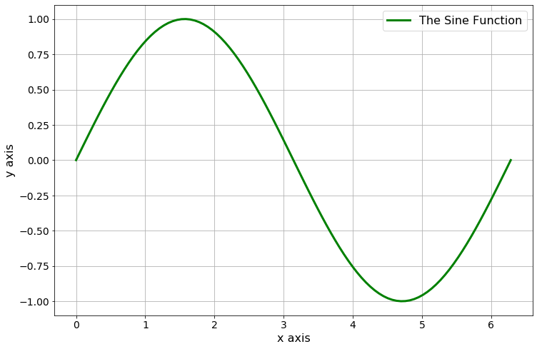
Figure A.1: The sine function
Example A.46 Now let’s do a second example, but this time we want to show four different plots on top of each other. When you start a figure, matplotlib is expecting all of those plots to be layered on top of each other.(Note:For MATLAB users, this means that you do not need the hold on command since it is automatically “on.”)
import numpy as np
import matplotlib.pyplot as plt
# %matplotlib inline # you may need this in Jupyter Notebooks

# build the x and y values
x = np.linspace(0,1,100)
y0 = np.sin(2*np.pi*x)
y1 = np.cos(2*np.pi*x)
y2 = y0 + y1
y3 = y0 - y1

# plot each of the functions
# (notice that they will be on the same axes)
plt.plot(x, y0, 'b-.', label=r"$y_0 = \sin(2\pi x)$")
plt.plot(x, y1, 'r--', label=r"$y_1 = \cos(2\pi x)$")
plt.plot(x, y2, 'g:', label=r"$y_2 = y_0 + y_1$")
plt.plot(x, y3, 'k-', label=r"$y_3 = y_0 - y_1$")

# put in a grid, legend, title, and axis labels
plt.grid()
plt.legend()
plt.title("Awesome Title")
plt.xlabel('x axis label')
plt.ylabel('y axis label')
plt.show()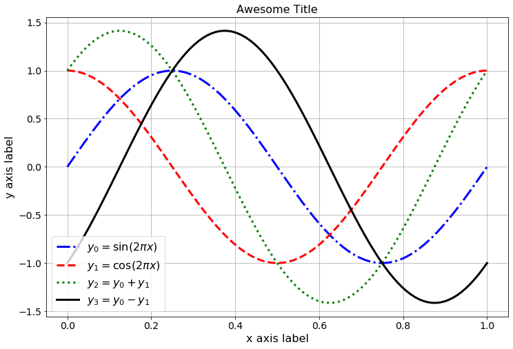
Figure A.2: Plots of the sine, cosine, and sums and differences.
Notice that the legend was placed automatically. There are ways to control the placement of the legend if you wish, but for now just let Python and matplotlib have control over the placement.
plot command can take several \((x, y)\) pairs in the same line of code. This can really shrink the amount of coding that you have to do when plotting several functions on top of each other.
# The next line of code does all of the plotting of all
# of the functions.  Notice the order: x, y, color and
# line style, repeat
import numpy as np
import matplotlib.pyplot as plt
x = np.linspace(0,1,100)
y0 = np.sin(2*np.pi*x)
y1 = np.cos(2*np.pi*x)
y2 = y0 + y1
y3 = y0 - y1
plt.plot(x, y0, 'b-.', x, y1, 'r--', x, y2, 'g:', x, y3, 'k-')

plt.grid()
plt.legend([r"$y_0 = \sin(2\pi x)$",r"$y_1 = \cos(2\pi x)$",\
            r"$y_2 = y_0 + y_1$",r"$y_3 = y_0 - y_1$"])
plt.title("Awesome Title")
plt.xlabel('x axis label')
plt.ylabel('y axis label')
plt.show()
Figure A.3: A second plot of the sine, cosine, and sums and differences.
A.6.2 Subplots
It is often very handy to place plots side-by-side or as some array of plots. The subplots command allows us that control. The main idea is that we are setting up a matrix of blank plots and then populating the axes with the plots that we want.
Example A.48 Let’s repeat the previous exercise, but this time we will put each of the plots in its own subplot. There are a few extra coding quirks that come along with building subplots so we’ll highlight each block of code separately.
- First we set up the plot area with
plt.subplots(). The first two inputs to thesubplotscommand are the number of rows and the number of columns in your plot array. For the first example we will do 2 rows of plots with 2 columns – so there are four plots total. The last input for thesubplotscommand is the size of the figure (this is really just so that it shows up well in Jupyter Notebooks – spend some time playing with the figure size to get it to look right). - Then we build each plot individually telling
matplotlibwhich axes to use for each of the things in the plots. - Notice the small differences in how we set the titles and labels
- In this example we are setting the \(y\)-axis to the interval \([-2,2]\) for consistency across all of the plots.
# set up the blank matrix of plots
import numpy as np
import matplotlib.pyplot as plt
x = np.linspace(0,1,100)
y0 = np.sin(2*np.pi*x)
y1 = np.cos(2*np.pi*x)
y2 = y0 + y1
y3 = y0 - y1

fig, axes = plt.subplots(nrows = 2, ncols = 2, figsize = (10,5))

# Build the first plot
axes[0,0].plot(x, y0, 'b-.')
axes[0,0].grid()
axes[0,0].set_title(r"$y_0 = \sin(2\pi x)$")
axes[0,0].set_ylim(-2,2)
axes[0,0].set_xlabel("x")
axes[0,0].set_ylabel("y")

# Build the second plot
axes[0,1].plot(x, y1, 'r--')
axes[0,1].grid()
axes[0,1].set_title(r"$y_1 = \cos(2\pi x)$")
axes[0,1].set_ylim(-2,2)
axes[0,1].set_xlabel("x")
axes[0,1].set_ylabel("y")

# Build the first plot
axes[1,0].plot(x, y2, 'g:')
axes[1,0].grid()
axes[1,0].set_title(r"$y_2 = y_0 + y_1$")
axes[1,0].set_ylim(-2,2)
axes[1,0].set_xlabel("x")
axes[1,0].set_ylabel("y")

# Build the first plot
axes[1,1].plot(x, y3, 'k-')
axes[1,1].grid()
axes[1,1].set_title(r"$y_3 = y_0 - y_1$")
axes[1,1].set_ylim(-2,2)
axes[1,1].set_xlabel("x")
axes[1,1].set_ylabel("y")

fig.tight_layout()
plt.show()
The fig.tight_layout() command makes the plot labels a bit more readable in this instance (again, something you can play with).
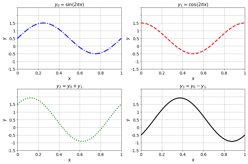
Figure A.4: An example of subplots
A.6.3 Logarithmic Scaling with semilogy, semilogx, and loglog
It is occasionally useful to scale an axis logarithmically. This arises most often when we’re examining an exponential function, or some other function, that is close to zero for much of the domain. Scaling logarithmically allows us to see how small the function is getting in orders of magnitude instead of as a raw real number. We’ll use this often in numerical methods.
import numpy as np
import matplotlib.pyplot as plt
x = np.linspace(0,500,1000)
y = 10**(-0.01*x)
fig, axis = plt.subplots(1,2, figsize = (10,5))

axis[0].plot(x,y, 'r')
axis[0].grid()
axis[0].set_title("Linearly scaled y axis")
axis[0].set_xlabel("x")
axis[0].set_ylabel("y")

axis[1].semilogy(x,y, 'k--')
axis[1].grid()
axis[1].set_title("Logarithmically scaled y axis")
axis[1].set_xlabel("x")
axis[1].set_ylabel("Log(y)")
plt.show()
It should be noted that the same result can be achieved using the yscale command along with the plot command instead of using the semilogy command. Pay careful attention to the subtle changes in the following code.
import numpy as np
import matplotlib.pyplot as plt
x = np.linspace(0,500,1000)
y = 10**(-0.01*x)
fig, axis = plt.subplots(1,2, figsize = (10,5))

axis[0].plot(x,y, 'r')
axis[0].grid()
axis[0].set_title("Linearly scaled y axis")
axis[0].set_xlabel("x")
axis[0].set_ylabel("y")

axis[1].plot(x,y, 'k--') # <----- Notice the change here
axis[1].set_yscale("log") # <----- And we added this line
axis[1].grid()
axis[1].set_title("Logarithmically scaled y axis")
axis[1].set_xlabel("x")
axis[1].set_ylabel("Log(y)")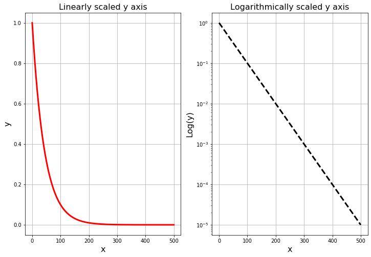
Figure A.5: An example of using logarithmic scaling.
subplots to put your plots side-by-side. Give appropriate labels, titles, etc.
A.7 Symbolic Python with sympy
In this section we will learn the tools necessary to do symbolic mathematics in Python. The relevant package is sympy (symbolic Python) and it works much like Mathematica, Maple, or MATLAB’s symbolic toolbox. That being said, Mathematica and Maple are designed to do symbolic computation in the fastest and best possible ways, so in some sense, sympy is a little step-sibling to these much bigger pieces of software. Remember: Python is free, and this is a book on numerical analysis – we will not be doing much symbolic work in this particular class, but these tools do occasionally come in handy.
Let’s import sympy in the usual way. We will use the nickname sp (just like we used np for numpy). This is not a standard nickname in the Python literature, but it will suffice for our purposes.
sympy and use the dir() command to see what functions are inside the sympy library.
sp.init_printing() after you load sympy you will get some nice LaTeX style output in your Jupyter Notebooks.
A.7.1 Symbolic Variables with symbols
When you are working with symbolic variables you have to tell Python that that’s what you’re doing. In other words, we actually have to type-cast the variables when we name them. Otherwise Python won’t know what to do with them – we need to explicitly tell it that we are working with symbols!
import sympy as sp
x = sp.Symbol('x') # note the capitalization
Now we’ll define the function \(f(x) = (x+2)^3\) and spend the next few examples playing with it.
f = (x+2)**3 # A symbolic function
print(f)
Notice that the output of these lines of code is not necessarily very nicely formatted as a symbolic expression. What we would really want to see is \(\displaystyle (x+2)^3\). If you include the code sp.init_printing() after you import the sympy library then you should get nice LaTeX style formatting in your answers.
# this line gives an error since it doesn't know
# which "sine" to use.
g = sin(x)
import sympy as sp
x = sp.Symbol('x')
g = sp.sin(x) # this one works
print(g)A.7.2 Symbolic Algebra
One of the primary purposes of doing symbolic programming is to do symbolic algebra (the other is typically symbolic calculus). In this section we’ll look at a few of the common algebraic exercises that can be handled with sympy.
import sympy as sp
x = sp.Symbol('x')
f = (x+2)**3
sp.expand(f) # do the multiplication to expand the polynomialimport sympy as sp
x = sp.Symbol('x')
h = x**2 + 4*x + 3
sp.factor(h) # factor this polynomialsympy package knows how to work with trigonometric identities. In this example we show how sympy expands \(\sin(a+b)\).
import sympy as sp
a, b = sp.symbols('a b')
j = sp.sin(a+b)
sp.expand(j, trig=True) # Trig identities are built in!import sympy as sp
x = sp.Symbol('x')
g = x**3 + 5*x**3 + 12*x**2 + 1
sp.simplify(g) # Simplify some algebraic expressionimport sympy as sp
x = sp.Symbol('x')
sp.simplify( sp.sin(x) / sp.cos(x)) # simplify a trig expression.Example A.58 (Symbolic Equation Solving) The primary goal of many algebra problems is to solve an equation. We will dedicate more time to algebraic equation solving later in this section, but this example gives a simple example of how it works in sympy.
import sympy as sp
x = sp.Symbol('x')
h = x**2 + 4*x + 3
sp.solve(h,x)
As expected, the roots of the function \(h(x)\) are \(x=-3\) and \(x=1\) since \(h(x)\) factors into \(h(x) = (x+3)(x-1)\).
A.7.3 Symbolic Function Evaluation
In sympy we cannot simply just evaluate functions as we would on paper. Let’s say we have the function \(f(x)= (x+2)^3\) and we want to find \(f(5)\). We would say that we “substitute 5 into f for x,” and that is exactly what we have to tell Python. Unfortunately we cannot just write f(5) since that would mean that f is a Python function and we are sending the number 5 into that function. This is an unfortunate double-use of the word “function,” but stop and think about it for a second: When we write f = (x+2)**3 we are just telling Python that f is a symbolic expression in terms of the symbol x, but we did not use def to define it as a function as we did for all other function.
import sympy as sp
x = sp.Symbol('x')
f = (x+2)**3
f(5) # This gives an error!
… but this is how it should be done:
import sympy as sp
x = sp.Symbol('x')
f = (x+2)**3
f.subs(x,5) # This actually substitutes 5 for x in f
A.7.4 Symbolic Calculus
The sympy package has routines to take symbolic derivatives, antiderivatives, limits, and Taylor series just like other computer algebra systems.
A.7.4.1 Derivatives
The diff command in sympy does differentiation: sp.diff(function, variable, [order]).
Take careful note that diff is defined both in sympy and in numpy. That means that there are symbolic and numerical routines for taking derivatives in Python …and we need to tell our instance of Python which one we’re working with every time we use it.
import sympy as sp
x = sp.Symbol('x') # Define the symbol x
f = (x+2)**3 # Define a symbolic function f(x) = (x+2)^3
df = sp.diff(f,x) # Take the derivative of f and call it "df"
print("f(x) = ", f)
print("f'(x) = ",df)
print("f'(x) = ", sp.expand(df))f.
import sympy as sp
x = sp.Symbol('x') # Define the symbol x
f = (x+2)**3 # Define a symbolic function f(x) = (x+2)^3
df = sp.diff(f,x,1) # first derivative
ddf = sp.diff(f,x,2) # second deriative
dddf = sp.diff(f,x,3) # third deriative
ddddf = sp.diff(f,x,4) # fourth deriative
print("f'(x) = ",df)
print("f''(x) = ",sp.simplify(ddf))
print("f'''(x) = ",sp.simplify(dddf))
print("f''''(x) = ",sp.simplify(ddddf))diff command is still the right tool. You just have to tell it which variable you’re working with.
import sympy as sp
x, y = sp.symbols('x y') # Define the symbols
f = sp.sin(x*y) + sp.cos(x**2) # Define the function
fx = sp.diff(f,x)
fy = sp.diff(f,y)
print("f(x,y) = ", f)
print("f_x(x,y) = ", fx)
print("f_y(x,y) = ", fy)sympy to give you the LaTeX code for the symbolic function so you can use it when you write about it.
import sympy as sp
x, y = sp.symbols('x y') # Define the symbols
f = sp.sin(x*y) + sp.cos(x**2) # Define the function
sp.latex(f)
A.7.4.2 Integrals
For integration, the sp.integrate tool is the command for the job: sp.integrate(function, variable) will find an antiderivative and sp.integrate(function, (variable, lower, upper)) will evaluate a definite integral.
The integrate command in sympy accepts a symbolically defined function along with the variable of integration and optional bounds. If the bounds aren’t given then the command finds the antiderivative. Otherwise it finds the definite integral.
import sympy as sp
x = sp.Symbol('x')
f = (x+2)**3
F = sp.integrate(f,x)
print(F)
The output of these lines of code is the expression \(\frac{x^{4}}{4} + 2 x^{3} + 6 x^{2} + 8 x\) which is indeed the antiderivative.
sympy package deals with the second variable just as it should.
import sympy as sp
x, y = sp.symbols('x y')
g = sp.sin(x*y) + sp.cos(x)
G = sp.integrate(g,x)
print(G)
It is apparent that sympy was sensitive to the fact that there was some trouble at \(y=0\) and took care of it with a piece wise function.
integrate command as a tuple. Furthermore, notice that we had to send the symbolic version of \(\pi\) instead of any other version (e.g. numpy).
import sympy as sp
x = sp.Symbol('x')
sp.integrate( sp.sin(x), (x,0,sp.pi))sympy. It is two lower-case O’s next to each other: oo. It kind of looks like and infinity I suppose.
import sympy as sp
x = sp.Symbol('x')
sp.integrate( sp.exp(-x**2) , (x, -sp.oo, sp.oo))
A.7.4.3 Limits
The limit command in sympy takes symbolic limits: sp.limit(function, variable, value, [direction])
The direction (left or right) is optional and if you leave it off then the limit is considered from both directions.
import sympy as sp
x = sp.Symbol('x')
sp.limit( sp.sin(x)/x, x, 0)diff command gives us the same thing using == …warning!
import sympy as sp
x = sp.Symbol('x')
f = (x+2)**3
print(sp.diff(f,x))
h = sp.Symbol('h')
df = sp.limit( (f.subs(x,x+h) - f) / h , h , 0 )
print(df)
print(df == sp.diff(f,x))
# notice that these are not "symbolically" equal
print(df == sp.expand(sp.diff(f,x))) # but these are
Notice that when we check to see if two symbolic functions are equal they must be in the same exact symbolic form. Otherwise sympy won’t recognize them as actually being equal even though they are mathematically equivalent.
Exercise A.23 Define the function \(f(x) = 3x^2 + x\sin(x^2)\) symbolically and then do the following:
- Evaluate the function at \(x=2\) and get symbolic and numerical answers.
- Take the first and second derivative
- Take the antiderivative
- Find the definite integral from 0 to 1
- Find the limit as \(x\) goes to 3
A.7.4.4 Taylor Series
The sympy package has a tool for expanding Taylor Series of symbolic functions: sp.series( function, variable, [center], [num terms]).
The center defaults to \(0\) and the number of terms defaults to \(5\).
import sympy as sp
x = sp.Symbol('x')
sp.series( sp.exp(x),x)
import sympy as sp
x = sp.Symbol('x')
sp.series( sp.exp(x), x, 1, 3) # expand at x=1 (3 terms)Finally, if we want more terms then we can send the number of desired
terms to the series command.
import sympy as sp
x = sp.Symbol('x')
sp.series( sp.exp(x), x, 0, 3) # expand at x=0 and give 3 terms
A.7.5 Solving Equations Symbolically
One of the big reasons to use a symbolic toolboxes such as sympy is to solve algebraic equations exactly. This isn’t always going to be possible, but when it is we get some nice results. The solve command in sympy is the tool for the job: sp.solve( equation, variable )
The equation doesn’t actually need to be the whole equation. For any equation-solving problem we can always re-frame it so that we are solving \(f(x) = 0\) by subtracting the right-hand side of the equation to the left-hand side. Hence we can leave the equal sign and the zero off and sympy understands what we’re doing.
import sympy as sp
x = sp.Symbol('x')
sp.solve( x**2 - 2, x)import sympy as sp
x = sp.Symbol('x')
sp.solve( x**4 - x**2 - 1, x)Run the code yourself to see the output. In nicer LaTeX style formatting, the answer is
\[\left[ - i \sqrt{- \frac{1}{2} + \frac{\sqrt{5}}{2}}, \ i \sqrt{- \frac{1}{2} + \frac{\sqrt{5}}{2}}, \ - \sqrt{\frac{1}{2} + \frac{\sqrt{5}}{2}}, \ \sqrt{\frac{1}{2} + \frac{\sqrt{5}}{2}}\right]\]
Notice that sympy has no problem dealing with the complex roots.
In the previous example the answers may be a bit hard to read due to their symbolic form. This is particularly true for far more complicated equation solving problems. The next example shows how you can loop through the solutions and then print them in decimal form so they are a bit more readable.
N command to convert from symbolic to numerical.
import sympy as sp
x = sp.Symbol('x')
soln = sp.solve( x**4 - x**2 - 1, x)
for j in range(0, len(soln)):
    print(sp.N(soln[j]))
The N command gives a numerical approximation for a symbolic expression (this is taken straight from Mathematica!).
When you want to solve a symbolic equation numerically you can use the nsolve command. This will do something like Newton’s method in the background. You need to give it a starting point where it can look for you the solution to your equation: sp.nsolve( equation, variable, intial guess )
nsolve will search for the solution near \(x=1\).
import sympy as sp
x = sp.Symbol('x')
ExactSoln = sp.solve(x**3 - x**2 - 2, x) # symbolic solution
print(ExactSoln)
Run the code yourself to see the exact solution. In nicer LaTeX style formatting the answer is: \[\begin{aligned} \left[ \frac{1}{3} + \left(- \frac{1}{2} - \frac{\sqrt{3} i}{2}\right) \sqrt[3]{\frac{\sqrt{87}}{9} + \frac{28}{27}} + \frac{1}{9 \left(- \frac{1}{2} - \frac{\sqrt{3} i}{2}\right) \sqrt[3]{\frac{\sqrt{87}}{9} + \frac{28}{27}}}, \right. \\ \frac{1}{3} + \frac{1}{9 \left(- \frac{1}{2} + \frac{\sqrt{3} i}{2}\right) \sqrt[3]{\frac{\sqrt{87}}{9} + \frac{28}{27}}} + \left(- \frac{1}{2} + \frac{\sqrt{3} i}{2}\right) \sqrt[3]{\frac{\sqrt{87}}{9} + \frac{28}{27}}, \\ \left. \frac{1}{9 \sqrt[3]{\frac{\sqrt{87}}{9} + \frac{28}{27}}} + \frac{1}{3} + \sqrt[3]{\frac{\sqrt{87}}{9} + \frac{28}{27}}\right]\end{aligned}\] which is rather challenging to read. We can give all of the floating point approximations with the following code.
import sympy as sp
x = sp.Symbol('x')
ExactSoln = sp.solve(x**3 - x**2 - 2, x) # symbolic solution
print("First Solution: ",sp.N(ExactSoln[0]))
print("Second Solution: ",sp.N(ExactSoln[1]))
print("Third Solution: ",sp.N(ExactSoln[2]))
If we were only looking for the floating point real solution near \(x=1\) then we could just use nsolve.
import sympy as sp
x = sp.Symbol('x')
NumericalSoln = sp.nsolve(x**3 - x**2 - 2, x, 1) # solution near x=1
print(NumericalSoln)A.7.6 Symbolic Plotting
In this final section we will show how to make plots of symbolically defined functions. Be careful here. There are times when you want to plot a symbolically defined function and there are times when you want to plot data: sp.plot( function, (variable, left, right) )
It is easy to get confused since they both use the plot function in their own packages (sympy and matplotlib respectively).
Note: For MATLAB users, the sympy.plot command is similar to MATLAB’s ezplot command or fplot command.
In numerical analysis we do not often need to make plots of symbolically defined functions. There is more that could be said about sympy’s plotting routine, but since it won’t be used often in this text it doesn’t seem necessary to give those details here. When you need to make a plot just make a careful consideration as to whether you need a
symbolic plot (with sympy) or a plot of data points (with matplotlib).
import sympy as sp
x = sp.Symbol('x')
f = (x+2)**3
sp.plot(f,(x,-5,2))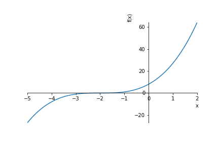
Figure A.6: A plot of a symbolically defined function.
Example A.76 Multiple plots can be done at the same time with the sympy.plot command.
import sympy as sp
x = sp.Symbol('x')
f = (x+2)**3
g = 20*sp.cos(x)
sp.plot(f, g, (x,-5,2))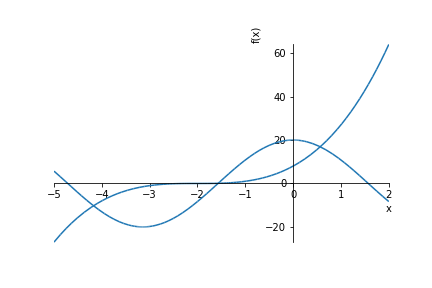
Figure A.7: A second plot of symbolically defined functions.
Actually, it is still an open mathematical question that every integer seed will converge to 1. The Collatz sequence has been checked for many millions of initial seeds and they all converge to 1, but there is no mathematical proof that it will always happen.↩︎