6 Partial Differential Equations

6.1 Intro to PDEs

“When you open the toolkit of differential equations you see the hammers and saws of engineering and physics for the past two centuries and for the foreseeable future.”
–Benoit Mandelbrot

Partial differential equations (PDEs) are differential equations involving the partial derivatives of an unknown multivariable function. The study of PDEs is highly motivated f3by physics. In most of this chapter we will examine two classical problems from physics: heat transport phenomenon and wave phenomenon. Don’t think, however, that just because we’re focusing only on these two primary examples that this is the extent of the utility of PDEs. Basically every scientific field has been impacted by (or has directly impacted) the study of PDEs. Any phenomenon that can be modeled via the change in multiple dimensions (and time) is likely governed by a PDE model. Some common phenomena that are modeled by PDEs are:

heat transport
- The heat equation models heat energy (temperature) diffusing through a metal rod or a solid body
diffusion of a concentrated substance
- The diffusion equation is a PDE model for the diffusion of smells, contaminants, or the motion of a solute
wave propagation
- The wave equation is a PDE that can be used to model the standing waves on a guitar string, the waves on lake, or sound waves traveling through the air
traveling waves
- The traveling wave equation is a PDE that can be used to model pulses of light propagating through a fiber optic cable or regions of high density traffic moving along a highway.
quantum mechanics
- The wave functions of quantum mechanics are described by a PDE called the Schrodinger Equation.
electro-magnetism
- Maxwell’s Equations are a system of PDEs describing the relationships between electricity and magnetism.
fluid flow
- The Navier-Stokes equations are a system of PDEs that model fluids in three dimensions – including turbulent flow.
- Darcy’s Law and Richard’s equation are PDE models for the motion of fluids moving through saturated and unsaturated soils.
stress and strain in structures
- The Linear Elasticity equation is a PDE that models the stresses in a solid body (like a bridge or a building) under load.
spatial patterns
- Solutions to the Helmholtz equation are known for exhibiting Turing patterns which are patterns like leopard spots or zebra stripes.
… and many more …

In many cases we are interested in ultimately solving PDEs in terms of our usual three spatial dimensions along with an extra dimension for time. However, in many cases we don’t have to work with all three spatial dimensions (like if the domain is much larger in one or two directions versus the others) or in some cases (like in linear elasticity) we don’t need to worry about time.

So what is a Partial Differential Equation?

Definition 6.1 (Partial Differential Equation) A partial differential equation (PDE) is an equation that relates a function and its partial derivatives. Typically we use the function name $u$ for the unknown function, and in most cases that we consider in this book we are thinking of $u$ as a function of time $t$ as well as one, two, or three spatial dimensions $x$, $y$, and $z$.

Specific examples of some common PDEs are:

In one spatial dimension the “heat equation” takes the form \[ \frac{\partial u}{\partial t} = D \frac{\partial^2 u}{\partial x^2}. \] This PDE states that the time derivative of the function $u$ is proportional to the second derivative with respect to the spatial dimension $x$. This PDE can be used to model the time evolution of temperature in a heated one-dimensional rod. To see a video introduction to the heat equation go to https://youtu.be/uV-96o8RwOI.
In three dimensions the heat equation takes the form \[ \frac{\partial u}{\partial t} = D\left( \frac{\partial^2 u}{\partial x^2} + \frac{\partial^2 u}{\partial y^2} + \frac{\partial^2 u}{\partial z^2} \right). \] This PDE states that the time derivative of $u$ is proportional to the sum of the three spatial second derivatives. This PDE can be used to model the time evolution of temperature in a heated three-dimensional object.
As a third example, consider the Laplace equation \[ \frac{\partial^2 u}{\partial x^2} + \frac{\partial^2 u}{\partial y^2} + \frac{\partial^2 u}{\partial z^2} = 0. \] This PDE states that the sum of the three second order derivatives is always zero. The Laplace equation gives the shape of an object that has minimum surface area while fixed to some boundary (like a soap bubble attached to a wire frame).
Finally, consider the three dimensional wave equation \[ \frac{\partial^2 u}{\partial t^2} = k\left( \frac{\partial^2 u}{\partial x^2} + \frac{\partial^2 u}{\partial y^2}+ \frac{\partial^2 u}{\partial z^2} \right). \] This PDE states that the acceleration at a point is proportional to the sum of the spatial second derivatives. The wave equation can be used to model the propagation of a sound wave through the air. For a video introduction to the wave equation go to https://youtu.be/hPcH22-ap9o.

There is a wealth of wonderful theory for finding analytic solutions to many special classes of PDEs. However, most PDEs simply do not easily lend themselves to analytic solutions that we can write down in terms of the regular mathematical operations of sums, products, powers, roots, trigonometric functions, logarithms, etc. Just like with ODEs, the trouble comes in that you are ultimately trying to integrate to solve the PDE, and we know that finding an antiderivative is usually an impossible task!

Recall that numerical solutions to ODEs were approximations of the value of the unknown function at every time. Similarly, numerical solutions to PDEs are going to be approximations of the value of the unknown function at every time AND at every point in the spatial domain.

What we’ll cover in this chapter will include one primary and powerful technique for approximating solutions to PDEs: the finite difference method. There are many other techniques for approximating solutions to PDEs, and the field of numerical PDEs is still an active area of mathematical and scientific research. For a quick video introduction to numerical PDEs go to https://youtu.be/_W7srt0hghY.

Lastly, since PDEs require a strong background in the notions of multivariable calculus let’s at least start with an exercise that should jog your memory about such things as the partial derivative, the gradient, and the divergence operators.

Exercise 6.1 With your partner answer each of the following questions. The main ideas in this problem should be review from multivariable calculus. If you and your partner are stuck then ask another group.

What is a partial derivative (explain geometrically)
What is the gradient of a function? What does it tell us physically or geometrically? If $u(x,y)=x^2+\sin(xy)$ then what is $\nabla u$?
What is the divergence of a vector-valued function? What does it tell us physically or geometrically? If $F(x,y)=\left< \sin(xy), x^2+y^2\right>$ then what is $\nabla \cdot F$?
If $u$ is a function of $x$, $y$, and $z$ then what is $\nabla \cdot \nabla u$?

6.2 Solutions to PDEs

Example 6.1 If we were to claim that $x(t) = 7e^{3t}$ is a solution to the ordinary differential equation $\frac{dx}{dt} = 3x$ with $x(0) = 7$ then you could easily check that the claim was true by doing two things:

Check that the proposed solution matches the initial condition. In this example we see that $x(0) = 7e^{3 \cdot 0} = 7 \quad \checkmark.$
Check that the function satisfies the differential equation. In other words, substitute the function $x(t)$ into the differential equation $x' = 3x$ and verify that the equal sign is actually true. In this case, $x' = 3\cdot 7e^{3t} = 3 x \quad \checkmark .$

Checking a solution to a differential equation amounts to substituting the function into the differential equation and the associated conditions and verifying that everything is true. Let’s do the same for some partial differential equations.

Exercise 6.2 Consider the PDE $u_t = D u_{xx}$ where $u(t,x)$ is the temperature of a long thin metal rod at time $t$ (in seconds) and spatial location $x$ (in meters).

Note: the symbol $u_t$ is quick shorthand for the partial derivative $\frac{\partial u}{\partial t}$ and $u_{xx}$ is a quick shorthand for the second partial derivative $\frac{\partial^2 u}{\partial x^2}$.

What are the units of the constant $D$?
For each of the following functions, test whether it is an analytical solution to this PDE by taking the first derivative with respect to time, the second derivative with respect to position, and substituting them into this equation to see if we get an identity (a true statement). If $D = 3$, which of these functions is a solution? Be able to defend your answer.
1. $u(t,x) = 4 x^3 + 6 t^2$
2. $u(t,x) = 7 x + 5$
3. $u(t,x) = 8 x^2 t$
4. $u(t,x) = e^{3 t + x}$
5. $u(t,x) = 6 e^{3 t + x} +5x - 2$
6. $u(t,x) = e^{-3t} + \sin (x)$
7. $u(t,x) = e^{3t} \sin (x)$
8. $u(t,x) = e^{-3t} \sin (x)$
9. $u(t,x) = 5 e^{-3t} \sin (x) + 6x + 7$
10. $u(t,x) = -4 e^{-3t} \sin (x) + 3t + 2$
11. $u(t,x) = e^{-2t} \sin (3x)$
12. $u(t,x) = e^{-12 t} \cos (3x)$
13. $u(t,x) = e^{-12 t} \cos (3x)+4x^2 + 8$
14. $u(t,x) = e^{-75 t} \cos (5x)$
15. $u(t,x) = 9 e^{-75 t} \cos (5x) + 2 x + 7$

Exercise 6.3 Consider the PDE $u_t = D u_{xx}$, and suppose that $D=4$. For each of the following functions, find the value of the parameter $a$ that will make the function solve the PDE, by taking derivatives and substituting them into the equation.

$u(t,x) = 6 e^{-8 t} \sin(ax)$
$u(t,x) = -5 e^{38 t} \cos(ax)$
$u(t,x) = 3 e^{at} \sin(5 x)$
$u(t,x) = 7 e^{at} \cos(2 x)$
$u(t,x) = a e^{-36t} \cos(3 x)$
$u(t,x) = a e^{-4t} \cos(6 x)$

Exercise 6.4 Consider again the PDE $u_t = D u_{xx}$. Is the function $u(t,x) = x^2 - t^3$ a valid solution for this differential equation? If so, what is the value of the constant $k$?

Calculate $u_t$ and $u_{xx}$ \[ u_t = \underline{\hspace{1in}} \quad \text{and} \quad u_{xx} = \underline{\hspace{1in}} \]
If the differential equation $u_t = Du_{xx}$ is to be satisfied then what equation must be true? \[ \underline{\hspace{1in}} = \underline{\hspace{1in}} \]
Is there a single value of $D$ that makes the PDE true with this proposed solution? If so, then we must have a solution to the PDE, if not then we must not have a solution to the PDE. Is $u(t,x)$ a solution to the equation $u_t = Du_{xx}$?

Exercise 6.5 The PDE $u_t = D u_{xx}$ can be seen as asking two questions: (1) the time derivative of the function $u(t,x)$ is related to the function $u$ itself, and (2) the second spatial derivative of the function $u(t,x)$ is related to the function $u$ itself.

What sort of function has the property that when you take the derivative you get a scaled version of the function back.
What sort of function has the property that when you take two derivatives you get a scaled version of the function back.
Based on your answers to parts (a) and (b), propose a function that might be a solution to the PDE.

Exercise 6.6 Is the function $u(t,x) = e^{-0.2t} \sin(\pi x)$ a solution to the PDE $u_t =Dk u_{xx}$? If this function is a solution to the PDE then what is the associated value of $D$?

Exercise 6.7 Is a scalar multiple of the function in the previous exercise also a solution to the PDE $u_t = D u_{xx}$ with the exact same value for $k$? Will this always be true? That is, if we have one solution $u(t,x)$ to the PDE $u_t = D u_{xx}$ then will $c u(t,x)$ be another solution for any real number $c$?

Exercise 6.8 When we studied ODEs we always had a starting point for a solution – the initial condition. In the case of a PDE we also need to have an initial condition, but the initial condition is associated with every point in the spatial domain. Hence, the initial condition is actually a function of $x$. In the previous exercise you found the $u(t,x) = e^{-0.2t} \sin(\pi x)$ is a solution to the PDE $u_t = D u_{xx}$. What is the initial condition that this solution satisfies? In other words, what is the function $u(t,x)$ at time $t=0$?

Exercise 6.9 Since we have both temporal and spatial variables in PDEs it stands to reason that we need conditions on both variables in order to get a unique solution to the PDE. For the PDE $u_t = D u_{xx}$ we already saw that $u(t,x) = e^{-0.2t} \sin(\pi x)$ is a solution to the PDE and the initial condition for that solution is $u(0,x) = \sin(\pi x)$. If we are solving the PDE on the domain $x \in [0,1]$ then what are the conditions that holds for all time at the points $x=0$ and $x=1$? These conditions are called boundary conditions.

Exercise 6.10 (Visualizing Solutions to PDEs) Solutions to PDEs are multivariable functions. In the previous few problems we have examined the heat equation $u_t = D u_{xx}$. The function $u$ is a function of time, $t$, and one spatial variable, $x$. We have several choices when we make a plot of this type of function. Implement and complete the blocks of code below to get three different visualizations of the solution $u(t,x) = e^{-0.2t} \sin(\pi x)$ on the domain $t \in [0,1]$ and $x \in [0,1]$.

The first idea is to show several discrete snapshots of time and to arrange the plots in an array so we can read from left to right to see the evolution in time.

import numpy as np
import matplotlib.pyplot as plt
u = lambda t, x: np.exp(-0.2*t) * np.sin(np.pi*x)
x = # code that gives 100 equally spaced points from 0 to 1 
t = # code that gives 16 equally spaced points from 0 to 10
fig, ax = plt.subplots(nrows=4,ncols=4)
counter = 0 # this counter will count through the times
for n in range(4):
    for m in range(4):
        ax[n,m].plot(??? , ???, 'b') # plot x vs u(t[counter],x)
        ax[n,m].grid()
        ax[n,m].set_ylim(0,1) # same axis for every plot
        ax[n,m].set_xlabel('x')
        ax[n,m].set_ylabel('u')
        ax[n,m].set_title("time="+np.str(t[counter]))
        counter += 1 # increment the counter
fig.tight_layout()        
plt.show()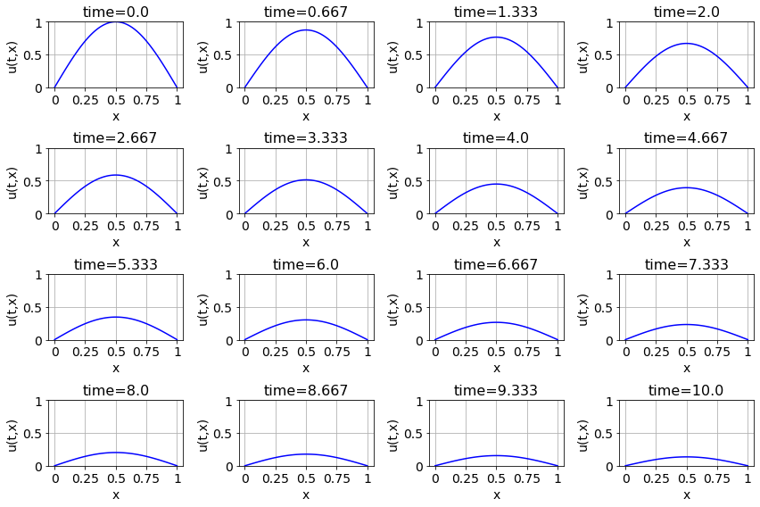

Figure 6.1: Time evolution of a solution to the PDE

A second idea for plotting the solution to a PDE is to give an interactive plot where we can use a slider to advance (or reverse) time.

import numpy as np
import matplotlib.pyplot as plt
from ipywidgets import interactive

u = lambda t, x: np.exp(-0.2*t) * (1*np.sin(1*np.pi*x))
x = np.linspace(0,1,100)

def plotter(T):
  plt.plot(x , u(T,x), 'b')
  plt.grid()
  plt.ylim(0,1)
  plt.show()

interactive_plot = interactive(plotter, T=(0,20,0.1))
interactive_plot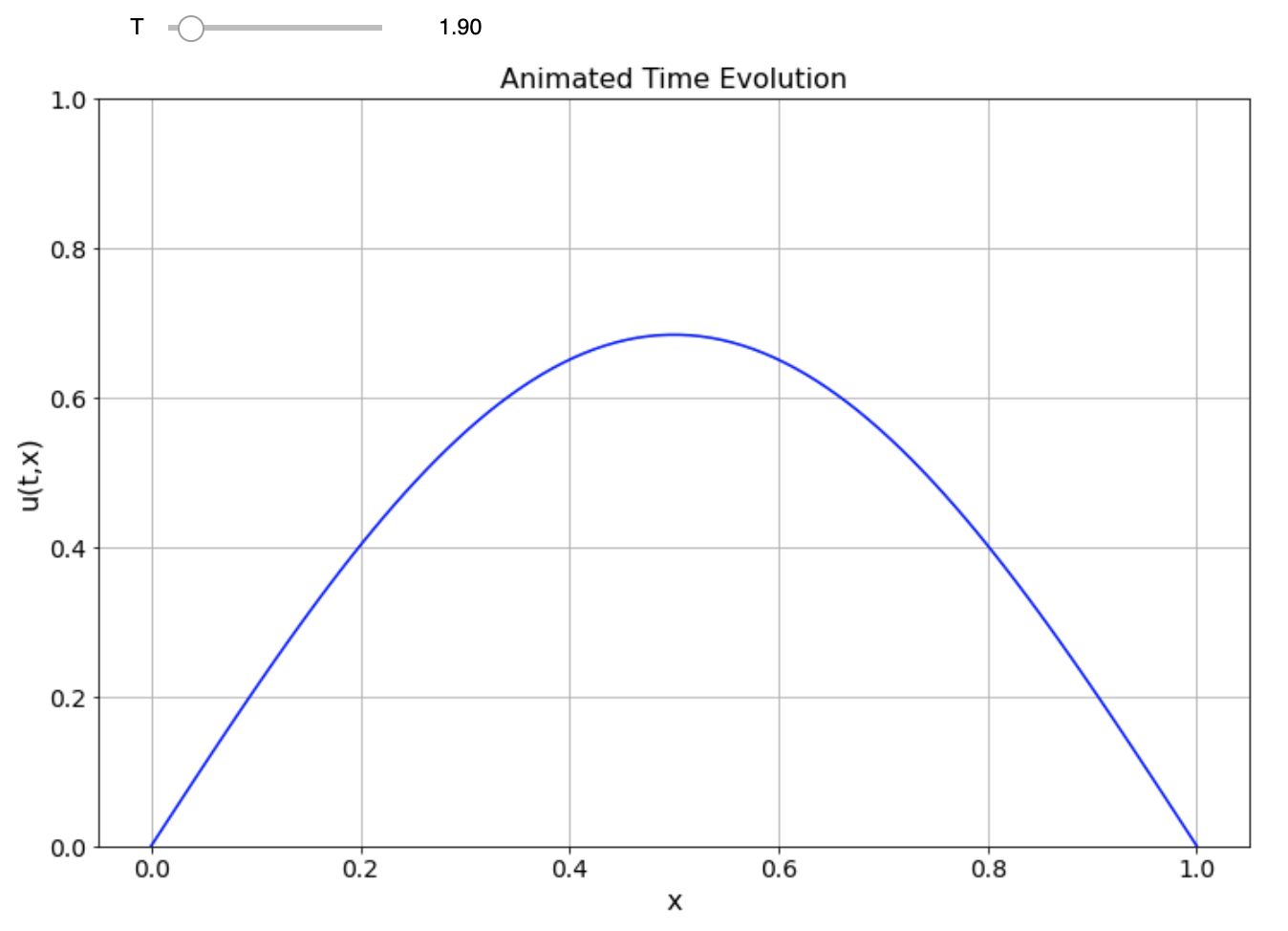

Figure 6.2: Snapshot of animated time evolution of a solution to the PDE

A third idea for plotting the solution to a PDE is to create a three dimensional plot with time on one axis, $x$ on the second axis, and $u$ on the vertical axis. To read this plot we start our eyes at $t=0$ and then scan down the $t$ axis. In this way we can see the whole time evolution of the PDE in one plot without animation. Of course, if the PDE had two or more spatial dimensions plus time then this sort of plot would not be feasible.

import numpy as np
import matplotlib.pyplot as plt
from mpl_toolkits.mplot3d import Axes3D
fig = plt.figure(figsize=(10,8))
ax = fig.gca(projection='3d') # gca stands for "Get Current Axis"
u = lambda t, x: np.exp(-0.2*t)*np.sin(np.pi*x)
x = np.linspace(0,1,25)
t = np.linspace(0,10,25)
T, X = np.meshgrid(t,x)
ax.plot_wireframe(T,X,u(T,X))
ax.set_xlabel('time')
ax.set_ylabel('x')
ax.set_zlabel('u(t,x)')
plt.show()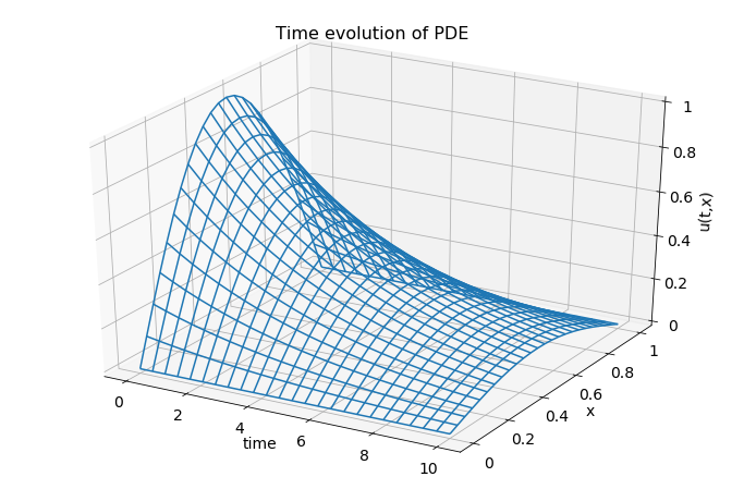

Figure 6.3: 3D plot showing the time evolution of the solution to the PDE.

A final idea is to use matplotlib.animation. Note that this method may only work well with the Google Colab environment.

import numpy as np
import matplotlib.pyplot as plt
from matplotlib import animation, rc
from IPython.display import HTML

u = lambda t, x: np.exp(-0.2*t)*np.sin(np.pi*x)
x = np.linspace(0,1,25)
t = np.linspace(0,10,101)

fig, ax = plt.subplots()
plt.close()
ax.grid()
ax.set_xlabel('x')
ax.set_xlim(( 0, 1))
ax.set_ylim(( 0, 1))
frame, = ax.plot([], [], linewidth=2, linestyle='--')

def animator(N):
  U = u(t[N],x)
  ax.set_title('Time='+str(t[N]))
  frame.set_data(x,U)
  return (frame,)

PlotFrames = range(0,len(t),1) 
anim = animation.FuncAnimation(fig, 
                               animator, 
                               frames=PlotFrames, 
                               interval=100, 
                              )
rc('animation', html='jshtml') # embed in the HTML for Google Colab
anim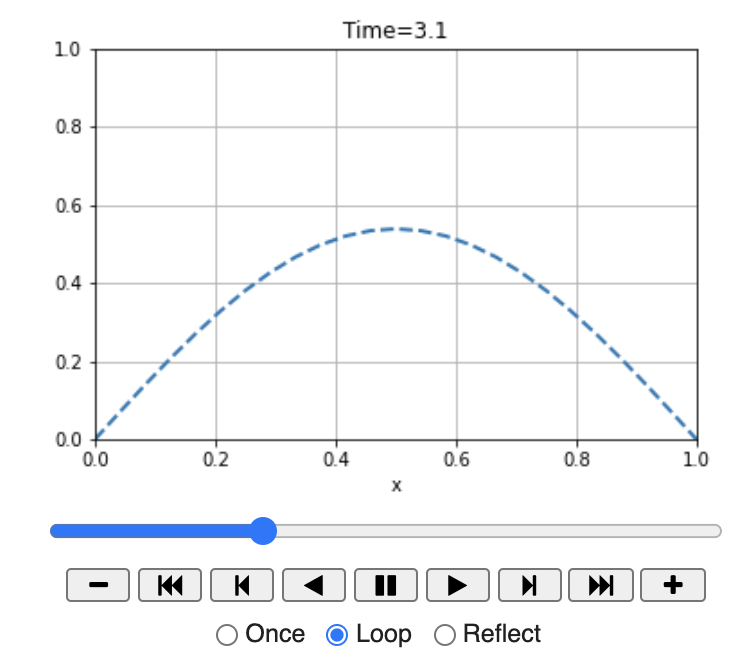

Figure 6.4: Snapshot of an animation applet showing the time evolution of the solution to the PDE.

Exercise 6.11 In the previous problem you built several plots of the function $u(t,x) = e^{-0.2t} \sin(\pi x)$ as a solution to the heat equation $u_t = D u_{xx}$.

Based on the plots, why do you think the equation $u_t = D u_{xx}$ called the “heat equation?” That is, why do the solutions look like dissipating heat?
What is the limit \[ \lim_{t \to \infty} u(t,x)? \] Explain why your answer makes sense if we are solving an equation, called the “heat equation,” that models the diffusion of heat through an object. Hint: think of this object as a long thing metal rod and take note that the boundary conditions are both 0.

Exercise 6.12 Propose another solution to the PDE $u_t = D u_{xx}$ that exactly matches the boundary conditions $u(t,0)=0$ and $u(t,1)=0$ for all time $t$ AND exactly the same value for $D$ as with the function $u(t,x) = e^{-0.2t} \sin(\pi x)$. What is the new initial condition associated with your new solution?

Hint: You may want to start with a function of the form $u(t,x) = e^{at} \sin( bx)$ and then determine values of $a$ and $b$ that will satisfy all of the required conditions.

Exercise 6.13 We now have two solutions to the PDE $u_t = D u_{xx}$ that satisfy both the PDE and the boundary conditions $u(t,0) = 0$ and $u(t,1)=0$.

Prove that the sum of the two solutions also satisfies the PDE and the same boundary conditions? If so, then the sum appears to be another valid solution to the PDE.
What is the initial condition associated with the new solution you found in part (a)?
Use the code that you built above to show the time evolution of your new solution.

Let’s take stock of what we’ve investigated thus far.

Theorem 6.1 If $u_0(t,x)$ and $u_1(t,x)$ are both solutions to the PDE $u_t = D u_{xx}$ matching the same boundary conditions $u(t,0) = u(t,1) = 0$ then for real scalars $c_0$ and $c_1$ the function $c_0 u_0(t,x) + c_1 u_1(t,x)$ is another solution to the PDE matching the same boundary conditions but perhaps having a different initial condition.

Exercise 6.14 Prove the previous theorem. Then extend the theorem to show that if there are many functions that satisfy $u_t = D u_{xx}$ and the boundary conditions $u(t,0) = u(t,1) = 0$ then the sum of all of the functions is also a solution and also satisfies the boundary conditions.

Exercise 6.15 Propose several solutions to the PDE $u_t = D u_{xx}$ with the boundary conditions $u(t,0) = 0$ and $u_x(t,1) = 0$. That is to say that the function $u(t,x)$ is $0$ at $x=0$ and the derivative of $u$ with respect to $x$ at $x=1$ is 0 (there is a horizontal tangent line to the function $u$ at $x=1$ for all times $t$). Then use your plotting code to verify that your solution satisfies the boundary conditions and visually shows the diffusion of heat as time evolves.

At this point we have a good notion of what the solutions to the PDE $u_t = D u_{xx}$ look and behave like. Now let’s ramp this up to two spatial dimensions.

Exercise 6.16 Leverage what you learned in the previous exercises to propose a function $u(t,x,y)$ that solves the equation \[ u_t = D \left( u_{xx} + u_{yy} \right) \] on the domain $x \in [0,1]$ and $y \in [0,1]$ with $D=1$, the boundary conditions $u(t,0,y) = 0$, $u(t,1,y) = 0$, $u(t,x,0)=u(t,x,1)=0$, and the initial condition $u(0,x,y) = \sin(\pi x) \sin(\pi y)$ (shown in Figure 6.5). Then use the code below to show the time evolution of your solution.

import numpy as np
import matplotlib.pyplot as plt
from ipywidgets import interactive

u = lambda t, x, y: # your function goes here
x, y = np.meshgrid( np.linspace(0,1,25), np.linspace(0,1,25) )

def plotter(T):
    fig = plt.figure(figsize=(15,12))
    ax = fig.gca(projection='3d')
    z = u(T,x,y)
    ax.plot_surface(x,y,z)
    ax.set_xlabel('x')
    ax.set_ylabel('y')
    ax.set_zlabel('u(t,x,y)')
    ax.set_zlim(0,1)
    plt.show()

interactive_plot = interactive(plotter, T = (0,10,0.1) )
interactive_plot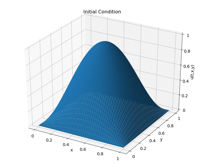

Figure 6.5: Initial condition

Exercise 6.17 Prove that the function $u(t,x,y) = e^{-0.2t} \sin(\pi x) \sin(\pi y)$ is a solution to the two dimensional heat equation $u_t = D(u_{xx} + u_{yy})$. Determine the value of $D$ for this particular solution. What are the boundary conditions and the initial condition?

Let’s move on to a different PDE: the wave equation.

Exercise 6.18 Consider the wave equation \[\frac{\partial^2 u}{\partial t^2} = c \frac{\partial^2 u}{\partial x^2}\] where $u$ is the height of the wave at time $t$.

What are the units of $c$?
Reading from left-to-right, the partial differential equation says that the second derivative of some function of $t$ is related to that same function. If you had to guess the type of function, what would you guess and why?
Reading from right-to-left, the partial differential equation says that the second derivative of some function of $x$ is related to that same function. If you had to guess the type of function, what would you guess and why?
Based on your guesses from parts (a) and (b), what type of function would think is a reasonable solution for the differential equation? Why?
If $u(0,x) = \sin(2\pi x)$ is the initial condition for the PDE and the boundary conditions are $u(t,0) = u(t,1) = 0$ then propose a solution that matches these conditions and make plots showing how the solution behaves over time.

Theorem 6.2 If the function $u(t,x)$ solves the 1D wave equation $u_{tt} = c u_{xx}$ then $u(t,x)$ likely has the functional form \[u(t,x) = \underline{\hspace{2in}}.\]

Exercise 6.19 Prove your hypotheses from the previous theorem.

Exercise 6.20 Make several plots of your solution showing the time evolution of the function. Examples of the plots are shown in Figures 6.6 and 6.7. Your plots may look different given the oscillation period and the initial condition.

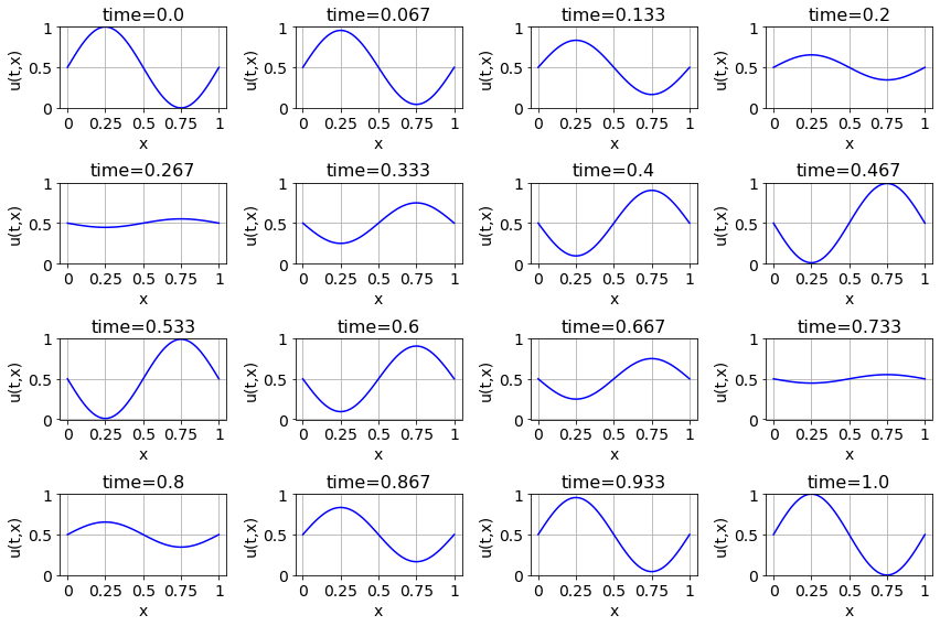
Figure 6.6: Time evolution of a solution to the wave equation.

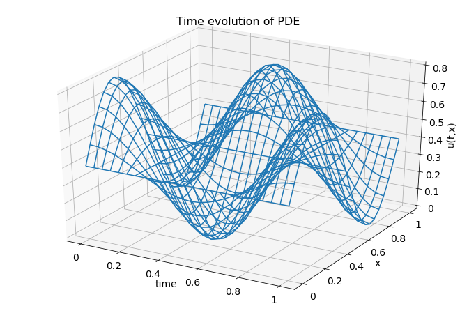
Figure 6.7: 3D plot of the time evolution of a solution to the wave equation.

Exercise 6.21 If $u_0(t,x)$ and $u_1(t,x)$ are both solutions the wave equation $u_{tt} = c u_{xx}$ matching boundary conditions $u(t,0) = u(t,1) = 0$, then is a linear combination of $u_0$ and $u_1$ also a solution that matches the particular boundary conditions?

Exercise 6.22 Consider the wave equation $u_{tt} = c ( u_{xx} + u_{yy})$ where $u(x,y,t)$ is the height (in centimeters) of a wave at time $t$ in seconds and spatial location $(x,y)$ (each in centimeters).

What are the units of the constant $c$?
For each of the following functions, test whether it is an analytical solution to this PDE by substituting the derivatives into the equation. If $c = 2$, which of these functions is a solution?
1. $u(t,x,y) = 3x + 2y + 5 t - 6$
2. $u(t,x,y) = 3x^2 + 2y^2 + 5 t^2 - 6$
3. $u(t,x,y) = \sin( 2 x) + \cos(3 y) + \sin(4t)$
4. $u(t,x,y) = \sin( 2 x) \cos(3 y) \sin(4t)$
5. $u(t,x,y) = \sin(3 x) \cos(4 y) \sin(10t)$
6. $u(t,x,y) = -6\sin( 3 x) \cos(4 y) \sin(10t)+2x -3y+9-12$
7. $u(t,x,y) = \cos(7 x) \cos(3 y) \cos(12t)$
8. $u(t,x,y) = \cos(5 x) \sin(12 y) \cos(13\sqrt{2}t)$
Make plots of the time evolution of the solutions from part (b). What phenomena do you observe in the plots?

Theorem 6.3 If the function $u(t,x,y)$ solves the 2D wave equation $u_{tt} = c \left( u_{xx} + u_{yy} \right)$ then $u(t,x,y)$ likely has the functional form \[u(t,x,y) = \underline{\hspace{2in}}.\]

Exercise 6.23 Prove your hypotheses from the previous theorem.

Exercise 6.24 Propose a solution to the wave equation $u_{tt} = c u_{xx}$ where $u(t,0) = 0$ and $u_x(t,1)=0$.

At this point we have only examined two PDEs, the heat and wave equations, and have proposed possible forms of the analytic solutions. These two particular PDEs have nice analytic solutions in terms of exponential and trigonometric functions so it isn’t terribly challenging to guess at the proper functional forms of the solutions. However, if we were to change the initial conditions, boundary conditions, or the differential equation by just a bit it may be more challenging to propose analytic solutions. It is not the purpose of this chapter to give a complete treatment of the analytic solutions to PDEs (not even the heat or wave equations). The purpose of what we just did was to build some intuition about the types of behaviors that we should expect from these prototypical PDEs. This way we will be able to determine if our numerical solutions in future sections are reasonable or not.

6.3 Boundary Conditions

When we were solving ODEs we typically needed initial conditions to tell us where the solutions starts at time $t=0$. Since PDEs require both spatial and temporal information we need to tell the differential equation how to behave both at time zero AND on the boundaries of the domain.

Definition 6.2 Let’s say that we want to solve a PDE with variable $t$ and $x$ on the domain $x \in [0,1]$.

The initial condition is a function $f(x)$ where $u(0,x) = f(x)$. In other words, we are dictating the value of $u$ at every point $x$ at time $t=0$.
The boundary conditions are restrictions for how the solution behaves at $x=0$ and $x=1$ (for this problem).
- If the value of the solution $u$ at the boundary is either a fixed value or a fixed function of time then we call the boundary condition a Dirichlet boundary condition. For example, $u(t,0) = 1$ and $u(t,1) = 5$ are Dirichlet boundary conditions for this domain. Similarly, the conditions $u(t,0) = 0$ and $u(t,1) = \sin(100\pi t)$ are also Dirichlet boundary conditions. Dirichlet boundary conditions give the exact value of $u$ the the boundary points.
- If the value of the solution $u$ depends on the flux of $u$ at the boundary then we call the boundary condition a Neumann boundary condition. For example, $\frac{\partial u}{\partial x}(t,0) = 0$ and $\frac{\partial u}{\partial x}(t,1) = 0$ are Neumann boundary conditions. They state that the flux of $u$ is fixed at the boundaries.

Let’s play with a couple problems that should help to build your intuition about boundary conditions in PDEs. Again, we will do this graphically instead of numerically.

Exercise 6.25 Consider solving the heat equation $u_t = D u_{xx}$ in 1 spatial dimension.

If a long thin metal rod is initially heated in the middle and the temperature at the ends of the rod is held fixed at 0 then the heat diffusion is described by the heat equation. What type of boundary conditions do we have in this setup? How can you tell? Draw a picture showing the expected evolution of the heat equation with these boundary conditions.
What if we take the initial condition for the 1D heat equation to be $u(0,x) = \cos(2\pi x)$ and enforce the conditions $\frac{\partial u}{\partial x}\Big|_{x=0} = 0$ and $u(t,1) = 1$. What types of boundary conditions are these? Draw a collection of pictures showing the expected evolution of the heat equation with these boundary conditions.

Exercise 6.26 Consider solving the wave equation $u_{tt} = c u_{xx}$ in 1 spatial dimension.

If a guitar string is pulled up in the center and held fixed at the frets then the resulting vibrations of the string are described by the wave equation. What type of boundary conditions do we have in this setup? How can you tell? Draw a picture showing the expected evolution of the heat equation with these boundary conditions.
What if we take the initial condition for the 1D wave equation to be $u(0,x) = \cos(2\pi x)$ and enforce the conditions $\frac{\partial u}{\partial x}\Big|_{x=0} = 0$ and $u(t,1) = 1$. What types of boundary conditions are these? Draw a collection of pictures showing the expected evolution of the wave equation with these boundary conditions.

The next two problems should help you to understand some of the basic scenarios that we might wish to solve with the heat and wave equation.

Exercise 6.27 For each of the following situations propose meaningful boundary conditions for the 1D or 2D heat equation.

A thin metal rod 1 meter long is heated to $100^\circ$C on the left end and is cooled to $0^\circ$C on the right end. We model the heat transport with the 1D heat equation $u_t = Du_{xx}$. What are the appropriate boundary and initial conditions?
A thin metal rod 1 meter long is insulated on the left end so that the heat flux through that end is 0. The rod is held at a constant temperature of $50^\circ$C on the right end. We model the heat transport with the 1D heat equation $u_t = D u_{xx}$. What are the appropriate boundary conditions?
In a soil-science lab a column of packed soil is insulated on the sides and cooled to $20^\circ$C at the bottom. The top of the column is exposed to a heat lamp that cycles periodically between $15^\circ$C and $25^\circ$C and is supposed to mimic the heating and cooling that occurs during a day due to the sun. We model the heat transport within the column with the 1D heat equation $u_t = D u_{xx}$. What are the appropriate boundary conditions?
A thin rectangular slab of concrete is being designed for a sidewalk. Imagine the slab as viewed from above. We expect the right-hand side to be heated to $50^\circ$C due to radiant heating from the road and the left-hand side to be cooled to approximately $20^\circ$C due to proximity to a grassy hillside. The top and bottom of the slab are insulated with a felt mat so that the flux of heat through both ends is zero. We model the heat transport with the 2D heat equation $u_t = D(u_{xx} + u_{yy})$. What are the appropriate boundary conditions?

Exercise 6.28 For each of the following situations propose meaningful boundary conditions for the 1D and 2D wave equation.

A guitar string is held tight at both ends and plucked in the middle. We model the vibration of the guitar string with the 1D wave equation $u_{tt} = c u_{xx}$. What are the appropriate boundary conditions?
A rope is stretched between two people. The person on the left holds the rope tight and doesn’t move. The person on the right wiggles the rope in a periodic fashion completing one full oscillation per second. We model the waves in the rope with the 1D wave equation $u_{tt} = c u_{xx}$. What are the appropriate boundary conditions?
A rubber membrane is stretched taught on a rectangular frame. The frame is held completely rigid while the membrane is stretched from equilibrium and then released. We model the vibrations in the membrane with the 2D wave equation $u_{tt} = c (u_{xx} + u_{yy})$. What are the appropriate boundary conditions?

6.4 The Heat Equation

Thus far in this chapter we have supplied you with the PDEs and then we have built solutions, plots, initial conditions, and boundary conditions based on intuition and some knowledge of Calculus. Before going any further, however, we should give a clear derivation for where the heat equation comes from. For the sake of brevity (and simpler algebra) we will just give a derivation for the 1D heat equation. The 2D and 3D derivations are all quite similar.

The heat equation is also often called the diffusion equation since it models the diffusion (spreading out) of all sorts of things – e.g. heat, the density of molecules in a gos, the concentration of solute in a solvent. Let’s say that the density of some gas is distributed somehow along a line segment. If we divide the line segment into discrete adjacent intervals then random molecular motion would dictate that in a small discrete time steps half of the density in interval $n$ would move to the interval to the right, and half of the density would move to the interval to the left. Of course this assumption is only valid if the intervals are small enough so as to capture the distance that a bumped molecule will move in the time step. Mathematically we can express this simple assumptions of random molecular motion as \[\underbrace{u(t_{k+1},x_n) - u(t_k,x_n)}_{\text{change in density in interval n}} = \underbrace{\frac{1}{2} u(t_k,x_{n+1})}_{\text{in from the right}} - \underbrace{\frac{1}{2} u(t_k,x_n)}_{\text{out to the right}} + \underbrace{\frac{1}{2}u(t_k,x_{n-1})}_{\text{in from the left}} - \underbrace{\frac{1}{2}u(t_k,x_n)}_{\text{out to the left}} .\]

Rearranging we can write the previous equation as \[u(t_{k+1},x_n) - u(t_k,x_n) = \frac{1}{2} \left( u(t_k,x_{n+1}) - 2 u(t_k,x_n) + u(t_k,x_{n-1}) \right).\] We have seen enough discrete approximations of derivatives now that the next step should seem obvious (hopefully)! If we divide the left-hand side by $\Delta t$ then it appears to be a discrete approximation of a time derivative. If we divide the right-hand side by $\Delta x^2$ then it appears to be the discrete approximation of a second derivative in space. Of course we need to do our algebra correctly so we end up with the equation \[\frac{u(t_{k+1},x_n) - u(t_k,x_n)}{\Delta t} = \frac{\Delta x^2}{2\Delta t} \left( \frac{u(t_k,x_{n+1}) - 2 u(t_k,x_n) + u(t_k,x_{n-1})}{\Delta x^2} \right).\]

Finally, if we take the limits as the time step, $\Delta t$, and the length of the spatial intervals, $\Delta x$, get arbirarily small we get \[\frac{\partial u}{\partial t} = D \frac{\partial^2 u}{\partial x^2}\] where we have combined the coefficients on the right-hand side into the diffusion coefficient $D$.

If there was a mechanism forcing density into each of the small intervals then we would end up with the forced heat equation \[\frac{\partial u}{\partial t} = D \frac{\partial^2 u}{\partial x^2} + f(x).\] where the function $f(x)$ would model exactly how the density is being forced into each spatial point $x$. We’ll let $f(x) = 0$ for the majority of this section for simplicity, but you can modify any of the code that you write in this section to include a forcing term.

Derivations of the 2D and 3D diffusion equations are very similar. You should stop now and at least work out the details of the 2D heat equation.

In the remainder of this section we’ll use a technique called the finite difference method to build numerical approximations to solutions of the heat equation in 1D, 2D, and 3D.

For the sake of simplicity we will start by considering the time dependent heat equation in 1 spatial dimension with no external forcing function \[ \frac{\partial u}{\partial t} = D \frac{\partial^2 u}{\partial x^2}. \] The constant $D$ is the called the diffusivity (the rate of diffusion) so in terms of physical problems, if $D$ is small then the diffusion occurs slowly and if $D$ is large then the diffusion occurs quickly. Just as we did in Chapter 3 to approximate derivatives and integrals numerically, and also in Chapter 5 to approximate solutions to ODEs, we will start by partitioning the domain into finitely many pieces and we will partition time into finitely many pieces.

Exercise 6.29 In 1 spatial dimension, the heat equation is simply \[u_t = D u_{xx}.\] We want to build a numerical approximation to the function $u(t,x)$ for a given collection of initial and boundary conditions.

First we need to introduce some notation for the numerical solution. As you’ll see in a moment, there is a lot to keep track of in numerical PDEs so careful index and well-chosen notation is essential. Let $U_i^n$ be the approximation of the solution to $u(t,x)$ at the point $t=t_n$ and $x=x_i$ (since we have two variables we need to two indices). For example, $U_4^1$ is the value of the approximation at time $t_1$ and at the spatial point $x_4$.

Next we need to approximate both derivatives $u_t$ and $u_{xx}$ in the PDE using methods that we have used before. Now would be a good time to go back to Chapter 3 and refresh your memory for how we build approximations of derivatives.

Give an approximation of $u_t$ similar to Euler’s method \[ u_t \approx \frac{??? - ???}{???}. \]
Give an approximation of $u_{xx}$ using the approximation for the second derivative from Chapter 3 \[ u_{xx} \approx \frac{??? - ??? + ???}{???}. \]
Put your answers from parts (a) and (b) together using the 1D heat equation \[\frac{??? - ???}{\Delta t} = D \left( \frac{??? - ??? + ???}{\Delta x^2} \right).\] Be sure that your indexing is correct: the superscript $n$ is the index for time and the subscript $i$ is the index for space.
Rearrange your result from part (c) to solve for $U_i^{n+1}$: \[\begin{aligned} U_i^{n+1} = ??? + \frac{D \Delta t}{\Delta x^2} \left( ??? - ??? + ??? \right). \end{aligned}\] The iterative scheme which you just derived is called a finite difference scheme for the heat equation. Notice that the term on the left is the only term at the next time step $n+1$. So, for every spatial point $x_i$ we can build $U_i^{n+1}$ by evaluating the right-hand side of the finite difference scheme.
What is the expected order of the error for the approximation of the time derivative in the finite difference scheme from part (d)?
What is the expected order of the error for the approximation of the spatial second derivative in the finite difference scheme from part (d)?
The numerical errors made by using the finite difference scheme we just built come from two sources: from the approximation of the time derivative and from the approximation of the second spatial derivative. The total error is the sum of the two errors. Fill in the question marks in the powers of the following expression: \[ \text{Numerical Error} = \mathcal{O}(\Delta t^{???}) + \mathcal{O}(\Delta x^{???}). \]
Explain what the result from part (g) means in plain English?

There are many different finite difference schemes due to the fact that there are many different ways to approximate derivatives (See Chapter 3). One convenient way to keep track of which information you are using and what you are calculating in a finite difference scheme is to use a finite difference stencil image. Figure 6.8 shows the finite difference stencil for the approximation to the heat equation that you built in the previous exercise. In this figure we are showing that the function values $U_{i-1}^n$, $U_i^n$, and $U_{i+1}^n$ at the points $x_{i-1}$, $x_i$, and $x_{i+1}$ are being used at time step $t_n$ to calculate $U_i^{n+1}$. We will build similar stencil diagrams for other finite difference schemes throughout this chapter.

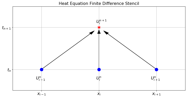
Figure 6.8: The finite difference stencil for the 1D heat equation.

Exercise 6.30 Now we want to implement your answer to part (d) of the previous exercise to approximate the solution to the following problem: \[\text{Solve: } u_t = 0.5u_{xx}\] with \[ x \in (0,1), \, u(0,x) = \sin(2 \pi x), \, u(t,0) = 0, \, \text{and} \, u(t,1) = 0.\] Some partial code is given below to get you started.

First we import the proper libraries, set up the time domain, and set up the spatial domain.

import numpy as np
import matplotlib.pyplot as plt
from ipywidgets import interactive

# Write code to give an array of times starting at t=0 and ending 
# at t=1.  Be sure that you use many points in the partition of 
# the time domain.  Be sure to either specify or calculate the 
# value of Delta t.

# Write code to give an array of x values starting at x=0 and 
# ending exactly at x=1. This is best done with the np.linspace() 
# command since you can guarantee that you end exactly at x=1.  
# Be sure to either specify or calculate the value of Delta x as
# part of your code. 

# The next two lines build two parameters that are of interest 
# for the finite difference scheme.
D = 0.5 # The diffusion coefficient for the heat equation given.
# The coefficient "a" appears in the finite difference scheme.
a = D*dt / dx**2 
print("dt=",dt,", dx=",dx," and D dt/dx^2=",a)

Next we build the array $U$ so we can store all of the approximations at all times and at all spatial points. The array will have the dimensions len(t) versus len(x). We then need to enforce the boundary conditions so for all times we fill the proper portions of the array with the proper boundary conditions. Lastly, we will build the initial condition for all spatial steps in the first time step.

U = np.zeros( (len(t),len(x)) )
U[:,0] = # left boundary condition
U[:,-1] = # right boundary condition
U[0,:] = # the function for the init. condition (should depend on x)

Now we step through a loop that fills the $U$ array one row at a time. Keep in mind that we want to leave the boundary conditions fixed so we will only fill indices 1 through -2 (stop and explain this). Be careful to get the indexing correct. For example, if we want $U_i^n$ we use U[n,1:-1], if we want $U_{i+1}^n$ we use U[n,2:], if we want $U_i^{n+1}$ we use U[n+1,1:-1], etc.

for n in range(len(t)-1):
    U[n+1,1:-1] = U[n,?:?] + a*( U[n,?:] - 2*U[n,?:?] + U[n,:?])

It remains to plot the solutions. One way to do this is with the ipywidgets.interactive tool. We first need to create a function which returns a plot at a particular time step. Then we call the function inside the interactive function. You could also use the matplotlib.animation function if you wish.

def plotter(Frame):
    plt.plot(x,U[Frame,:],'b')
    plt.grid()
    plt.ylim(-1,1)
    plt.show()
interactive_plot = interactive(plotter, Frame=(0,len(t)-1,1))
interactive_plot

Note: If you don’t want to do an interactive plot then you can produce several snapshots of the solutions with the following code.

for Frame in range(0,len(t),20): # ex: build every 20th frame
    plotter(Frame)

Exercise 6.31 You may have found that you didn’t get a sensible solution out for the previous problem. The point of this exercise is to show that value of $a = D\frac{\Delta t}{\Delta x^2}$ controls the stability of the finite difference solution to the heat equation, and furthermore that there is a cutoff for $a$ below which the finite difference scheme will be stable. Experiment with values of $\Delta t$ and $\Delta x$ and conjecture the values of $a = D \frac{\Delta t}{\Delta x^2}$ that give a stable result. Your conjecture should take the form:

If $a = D\frac{\Delta t}{\Delta x^2} < \underline{\hspace{0.5in}}$ then the finite difference solution for the 1D heat equation is stable. Otherwise it is unstable.

Exercise 6.32 Consider the one dimensional heat equation with diffusion coefficient $D=1$: \[ u_t = u_{xx}. \] We want to solve this equation on the domain $x \in (0,1)$ and $t\in (0,0.5)$ subject to the initial condition $u(0,x) = \sin(\pi x)$ and the boundary conditions $u(t,0)=u(t,1) = 0$.

Prove that the function $u(t,x) = e^{-\pi^2 t} \sin(\pi x)$ is a solution to this heat equation, satisfies the initial condition, and satisfies the boundary conditions.
Pick values of $\Delta t$ and $\Delta x$ so that you can get a stable finite difference solution to this heat equation. Plot your results on top of the analytic solution from part (a).
Now let’s change the initial condition to $u(0,x)=\sin(\pi x) + 0.1\sin(100 \pi x)$. Prove that the function $u(t,x) = e^{-\pi^2 t} \sin(\pi x) + 0.1 e^{-10^4\pi^2t}\sin(100\pi x)$ is a solution to this heat equation, matches this new initial condition, and matches the boundary conditions.
Pick values of $\Delta t$ and $\Delta x$ so that you can get a stable finite difference solution to this heat equation. Plot your results on top of the analytic solution from part (c).

Exercise 6.33 In any initial and boundary value problem such as the heat equation, the boundary values can either be classified as Dirichlet or Neumann type. In Dirichlet boundary conditions the values of the solution at the boundary are dictated specifically. So far we have only solved the heat equation with Dirichlet boundary conditions. In contrast, Neumann boundary conditions dictate the flux at the boundary instead of the value of the solution. Consider the 1D heat equation $u_t = u_{xx}$ with boundary conditions $u_x(t,0)=0$ and $u(t,1)=0$ with initial condition $u(0,x) = \cos(\pi x/2)$. Notice that the initial condition satisfies both boundary conditions: $\frac{d}{dx}(\cos(\pi \cdot x/2))\Big|_{x=0} = 0$ and $\cos(\pi \cdot 1/2)=0$. As the heat profile evolves in time the Neumann boundary condition $u_x(t,0)=0$ says that the slope of the solution needs to be fixed at 0 at the left-hand boundary.

Draw several images of what the solution to the PDE should look like as time evolves. Be sure that all boundary conditions are satisfied and that your solution appears to solve the heat equation.
The Neumann boundary condition $u_x(t,0) = 0$ can be approximated with the first order approximation \[ u_x(t_n,0) \approx \frac{U_1^n - U_0^n}{\Delta x}. \] If we set this approximation to 0 (since $u_x(t,0)=0$) and solve for $U_0^n$ we get an additional constraint at every time step of the numerical solution to the heat equation. What is this new equation.
Modify your 1D heat equation code to implement this Neumann boundary condition. Give plots that demonstrate that the Neumann boundary is indeed satisfied.

Exercise 6.34 Modify your 1D heat equation code to solve the following problems. For each be sure to classify the type of boundary conditions given. Notice that we are now using initial and boundary conditions where it would be quite challenging to built the analytic solution so we will only show numerical solutions. Be sure that you choose $\Delta t$ and $\Delta x$ so that your solution is stable.

Solve $u_t = 0.5 u_{xx}$ with $x \in (0,1)$, $u(0,x) = x^2$, $u(t,0) = 0$ and $u(t,1) = 1$.
Solve $u_t = 0.5 u_{xx}$ with $x \in (0,1)$, $u(0,x) = 1-\cos(\pi x/2)$, $u_x(t,0) = 0$ and $u(t,1) = 1$.
Solve $u_t = 0.5 u_{xx}$ with $x \in (0,1)$, $u(0,x) = \sin(2\pi x)$, $u(t,0) = 0$ and $u(t,1) = \sin(5\pi t)$.
Solve $u_t = 0.5 u_{xx}+x^2/100$ with $x \in (0,1)$, $u(0,x) = \sin(2\pi x)$, $u(t,0) = 0$ and $u(t,1) = 0$.

Now we transition to the two dimensional heat equation. Instead of thinking of this as heating a long metal rod we can think of heating a thin plate of metal (like a flat cookie sheet). The heat equation models the propagation of the heat energy throughout the 2D surface. In two spatial dimensions the heat equation is \[ \frac{\partial u}{\partial t} = D \left( \frac{\partial^2 u}{\partial x^2} + \frac{\partial^2 u}{\partial y^2} \right) \] or using subscript notation for the partial derivatives, \[ u_t = D\left( u_{xx} + u_{yy} \right). \]

Exercise 6.35 Let’s build a numerical solution to the 2D heat equation. We need to make a minor modification to our notation since there is now one more spatial dimension to keep track of. Let $U_{i,j}^n$ be the approximation to $u$ at the point $(t_n, x_i, y_j)$. For example, $U_{2,3}^4$ will be the approximation to the solution at the point $(t_4,x_2,y_3)$.

We already know how to approximate the time derivative in the heat equation: \[ u_t(t_{n+1}, x_i, y_j) \approx \frac{U_{i,j}^{n+1} - U_{i,j}^n}{\Delta t}. \] The new challenge now is that we have two spatial partial derivatives: one in $x$ and one in $y$. Use what you learned in Chapter 3 to write the approximations of $u_{xx}$ and $u_{yy}$. \[ u_{xx}(t_n,x_i,y_j) \approx \frac{??? - ??? + ???}{\Delta x^2} \] \[ u_{yy}(t_n,x_i,y_j) \approx \frac{??? - ??? + ???}{\Delta y^2} \] Take careful note that the index $i$ is the only one that changes for the $x$ derivative. Similarly, the index $j$ is the only one that changes for the $y$ derivative.
Put your answers to part (a) together with the 2D heat equation \[ \frac{U_{i,j}^{n+1} - U_{i,j}^n}{\Delta t} = D \left( \frac{??? - ??? + ???}{\Delta x^2} + \frac{??? - ??? + ???}{\Delta y^2} \right). \]
Let’s make one simplifying assumption. Choose the partition of the domain so that $\Delta x = \Delta y$. Note that we can usually do this in square domains. In more complicated domains we will need to be more careful. Simplify the right-hand side of your answer to part (b) under this assumption. \[ \frac{U_{i,j}^{n+1} - U_{i,j}^n}{\Delta t} = D \left( \frac{??? + ??? - ??? + ??? + ???}{???} \right). \]
Now solve your result from part (c) for $U_{i,j}^{n+1}$. Your answer is the explicit finite differene scheme for the 2D heat equation. \[ U_{i,j}^{n+1} = U_{???,???}^{???} + \frac{D \cdot ???}{???} \left( ??? + ??? - ??? + ??? + ??? \right) \]

The finite difference stencil for the 2D heat equation is a bit more complicated since we now have three indices to track. Hence, the stencil is naturally three dimensional. Figure 6.9 shows the stencil for the finite difference scheme that we built in the previous exercise. The left-hand subplot in the figure shows the five points used in time step $t_n$, and the right-hand subplot shows the one point that is calculated at time step $t_{n+1}$.

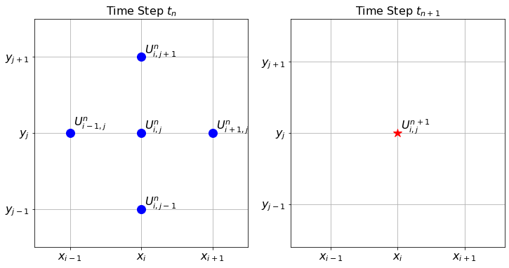
Figure 6.9: The finite difference stencil for the 2D heat equation.

Exercise 6.36 Now we need to implement the finite difference scheme that you developed in the previous problem. As a model problem, consider the 2D heat equation $u_t = D(u_{xx} + u_{yy})$ on the domain $(x,y) \in [0,1] \times [0,1]$ with the initial condition $u(0,x,y) = \sin(\pi x)\sin(\pi y)$, homogeneous Dirichlet boundary conditions, and $D=1$.¹³ Fill in the holes in the following code chunks.

First we import the proper libraries and set up the domains for $x$, $y$, and $t$.

import numpy as np
import matplotlib.pyplot as plt
from matplotlib import cm # this allows for color maps 
from ipywidgets import interactive

# Write code to build a linearly spaced array of x values 
# starting at 0 and ending at exactly 1
x = # your code here
y = x # This is a step that allows for us to have y = x 
# The consequence of the previous line is that dy = dx.
dx = # Extract dx from your array of x values.
# Now write code to build a linearly spaced array of time values 
# starting at 0 and ending at 0.25.
# You will want to use many more values for time than for space 
# (think about the stability conditions from the 1D heat equation).
t = # your code here
dt = # Extract dt from your array of t values

# Next we will use the np.meshgrid() command to turn the arrays of 
# x and y values into 2D grids of x and y values.  
# If you match the corresponding entries of X and Y then you get 
# every ordered pair in the domain.
X, Y = np.meshgrid(x,y)

# Next we set up a 3 dimensional array of zeros to store all of 
# the time steps of the solutions.
U = np.zeros( (len(t), len(x), len(y)))

Next we have to set up the boundary and initial conditions for the given problem.

U[0,:,:] = # initial condition depending on X and Y
U[:,0,:] = # boundary condition for x=0
U[:,-1,:] = # boundary condition for x=1
U[:,:,0] = # boundary condition for y=0
U[:,:,-1] = # boundary condition for y=1

We know that the value of $D \Delta t / \Delta x^2$ controls the stability of finite element methods. Therefore, the next step in our code is to calculate this value and print it.

D = 1
a = D*dt/dx**2
print(a)

Next for the part of the code that actually calculates all of the time steps. Be sure to keep the indexing straight. Also be sure that we are calculating all of the spatial indices inside the domain since the boundary conditions dictate what happens on the boundary.

for n in range(len(t)-1):
  U[n+1,1:-1,1:-1] = U[n,1:-1,1:-1] + \
    a*(U[n, ?:? , ?:?] + \
       U[n, ?:?, ?:?] - \
       4*U[n, ?:?, ?:?] + \
       U[n, ?:?, ?:?] + \
       U[n, ?:?, ?:?])

Finally, we just need to visualize the solution. Again we use the ipywidgets.interactive tool to build an interactive plot with time as the slider.

def plotter(Frame):
  fig = plt.figure(figsize=(12,10))
  ax = fig.gca(projection='3d')
  ax.plot_surface(X,Y,U[Frame,:,:], cmap=cm.coolwarm)
  ax.set_zlim(0,1)
  plt.show()

interactive_plot = interactive(plotter, Frame=(0,len(t)))
interactive_plot

Fill in all of the holes in the code and verify that your solution appears to solve a heat dissipation problem.

Theorem 6.4 In order for the finite difference solution to the 2D heat equation on a square domain to be stable then we need $D \Delta t / \Delta x^2 < \underline{\hspace{0.5in}}$.

Experiment with several parameters to imperically determine the bound.

Exercise 6.37 Time to do some experimentation with your new 2D heat equation code! Numerically solve the 2D heat equation with different boundary conditions (both Dirichlet and Neumann). Be prepared to present your solutions.

Exercise 6.38 Now solve the 2D heat equation on a rectangular domain. You will need to make some modifications to your code since it is unlikely that assuming that $\Delta x = \Delta y$ is a good assumption any longer. Again, be prepared to present your solutions.

6.5 Stability of the Heat Equation Solution

Exercise 6.39 (Sawtooth Errors) We have already seen that the 1D heat equation is stable if $D \Delta t / \Delta x^2 < 0.5$. The goal of this problem is to show what, exactly, occurs when we choose parameters in the unstable region. We’ll solve the PDE $u_t = u_{xx}$ on the domain $x \in [0,1]$ with initial conditions $u(0,x) = \sin(\pi x)$ then the analytic solution is $u(t,x) = e^{-\pi^2 t}\sin(\pi x)$. To build the spatial and temporal domains we will use x = np.linspace(0,1,21) and t = np.linspace(0,0.25,101). This means that $\Delta x = 0.05$ and $\Delta t = 0.0025$ so the ratio $D \Delta t / \Delta x^2 = 1 > 0.5$ (certainly in the unstable region). Solve the heat equation with finite differences using these parameters. Make plots of the approximate solution on top of the exact solution at time steps 0, 10, 20, 30, 31, 32, 33, 34, etc. Describe what you observe as the time step exceeds 30.

Exercise 6.40 Solve the 2D heat equation on the unit square with the following parameters:

A partition of 21 points in both the $x$ and $y$ direction.
301 points between 0 and 0.25 for time
An initial condition of $u(0,x,y) = \sin(\pi x) \sin(\pi y)$

What happens near time step number 70?

Exercise 6.41 What you saw in the previous two exercises is an example of a sawtooth error that occurs when a numerical solution technique for a PDE is unstable. Propose a conjecture for why this type of error occurs.

Theorem 6.5 Let’s summarize the stability criteria for the finite difference solutions to the heat equation.

In the 1D heat equation the finite difference solution is stable if $D \Delta t / \Delta x^2 < \underline{\hspace{0.5in}}$.
In the 2D heat equation the finite difference solution is stable if $D \Delta t / \Delta x^2 < \underline{\hspace{0.5in}}$ (assuming a square domain where $\Delta x = \Delta y$)
Propose a stability criterion for the 3D heat equation.

Exercise 6.42 Rewrite your finite difference code so that it produces an error message when the parameters will result in an unstable finite difference solution. Do the same for your 2D heat equation code.

It is actually possible to beat the stability criteria given in the previous exercises! What follows are two implicit methods that use a forward-looking scheme to help completely avoid unstable solutions. The primary advantage to these schemes is that we won’t need to pay as close attention to the ratio of the time step to the square of the spatial step. Instead, we can take time and spatial steps that are appropriate for the application we have in mind.

Exercise 6.43 (Implicit Finite Difference Scheme) For the 1D heat equation $u_t = D u_{xx}$ we have been finding the numerical solution using the explicit finite difference scheme \[\frac{U_i^{n+1} - U_i^n}{\Delta t} = D \frac{U_{i+1}^{n} - 2U_i^{n} + U_{i-1}^{n}}{\Delta x^2}\] where we approximate the time derivative with the usual forward difference and we approximate the spatial derivative with the usual centered difference. If, however, we use the spatial derivative at time step $n+1$ instead of time step $n$ we get the finite difference scheme \[\frac{U_i^{n+1} - U_i^n}{\Delta t} = D \frac{U_{i+1}^{n+1} - 2U_i^{n+1} + U_{i-1}^{n+1}}{\Delta x^2}.\] This may seem completely ridiculous since we don’t yet know the information at time step $n+1$ but some algebraic rearrangement shows that we can treat this as a system of linear equations which can be solved (using something like np.linalg.solve()) for the $(n+1)^{st}$ time step.

Before we start let’s define the coefficient $a = D \Delta t / \Delta x^2.$ This will save a little bit of writing in the coming steps.

Rearrange the new finite difference scheme so that all of the terms at the $(n+1)^{st}$ time step are on the left-hand side and all of the term at the $n^{th}$ time step are on the right-hand side. \[(\underline{\hspace{0.25in}}) U_{i-1}^{n+1} + (\underline{\hspace{0.5in}}) U_{i}^{n+1} + (\underline{\hspace{0.25in}}) U_{i-1}^{n+1} = \underline{\hspace{0.25in}} U_i^n\]
Now we’re going to build a very small example with only 6 spatial points so that you can clearly see the structure of the resulting linear system.
1. If we have 6 total points in the spatial grid ($x_0, x_1, \ldots, x_5$) then we have the following equations (fill in the blanks): \[\begin{aligned} (\text{for $x_1$: }) \quad \underline{\hspace{0.25in}} U_0^{n+1} + \underline{\hspace{0.5in}} U_1^{n+1} + \underline{\hspace{0.25in}} U_2^{n+1} &= \underline{\hspace{0.25in}} U_1^{n} \\ (\text{for $x_2$: }) \quad \underline{\hspace{0.25in}} U_1^{n+1} + \underline{\hspace{0.5in}} U_2^{n+1} + \underline{\hspace{0.25in}} U_3^{n+1} &= \underline{\hspace{0.25in}} U_2^{n} \\ (\text{for $x_3$: }) \quad \underline{\hspace{0.25in}} U_2^{n+1} + \underline{\hspace{0.5in}} U_3^{n+1} + \underline{\hspace{0.25in}} U_4^{n+1} &= \underline{\hspace{0.25in}} U_3^{n} \\ (\text{for $x_4$: }) \quad \underline{\hspace{0.25in}} U_3^{n+1} + \underline{\hspace{0.5in}} U_4^{n+1} + \underline{\hspace{0.25in}} U_5^{n+1} &= \underline{\hspace{0.25in}} U_4^{n} \\ \end{aligned}\]
2. Notice that we aready know $U_0^{n+1}$ and $U_5^{n+1}$ since these are dictated by the boundary conditions (assuming Dirichlet boundary conditions). Hence we can move these known quantities to the right-hand side of the equations and hence rewrite the system of equations as: \[\begin{aligned} (\text{for $x_1$: }) &\quad \underline{\hspace{0.5in}} U_1^{n+1} + \underline{\hspace{0.25in}} U_2^{n+1} = \underline{\hspace{0.25in}} U_1^{n} + \underline{\hspace{0.25in}} U_0^{n+1}\\ (\text{for $x_2$: }) &\quad \underline{\hspace{0.25in}} U_1^{n+1} + \underline{\hspace{0.5in}} U_2^{n+1} + \underline{\hspace{0.25in}} U_3^{n+1} = \underline{\hspace{0.25in}} U_2^{n} \\ (\text{for $x_3$: }) &\quad \underline{\hspace{0.25in}} U_2^{n+1} + \underline{\hspace{0.5in}} U_3^{n+1} + \underline{\hspace{0.25in}} U_4^{n+1} = \underline{\hspace{0.25in}} U_3^{n} \\ (\text{for $x_4$: }) &\quad \underline{\hspace{0.25in}} U_3^{n+1} + \underline{\hspace{0.5in}} U_4^{n+1} = \underline{\hspace{0.25in}} U_4^{n} + \underline{\hspace{0.25in}} U_5^{n+1} \\ \end{aligned}\]
3. Now we can leverage linear algebra and write this as a matrix equation. \[\begin{pmatrix} \underline{\hspace{0.25in}} & \underline{\hspace{0.25in}} & 0 & 0 \\ \underline{\hspace{0.25in}} & \underline{\hspace{0.25in}} & \underline{\hspace{0.25in}} & 0 \\ 0 & \underline{\hspace{0.25in}} & \underline{\hspace{0.25in}} & \underline{\hspace{0.25in}} \\ 0 & 0 & \underline{\hspace{0.25in}} & \underline{\hspace{0.25in}} \end{pmatrix}\begin{pmatrix} U_1^{n+1} \\ U_2^{n+1} \\ U_3^{n+1} \\ U_4^{n+1} \end{pmatrix} = \begin{pmatrix} U_1^{n} \\ U_2^{n} \\ U_3^{n} \\ U_4^{n} \end{pmatrix} + \begin{pmatrix} \underline{\hspace{0.25in}} U_0^{n+1} \\ 0 \\ 0 \\ \underline{\hspace{0.25in}} U_5^{n+1} \end{pmatrix}\]
At this point the structure of the coefficient matrix on the left and the vector sum on the right should be clear (even for more spatial points). It is time for us to start writing some code. We’ll start with the basic setup of the problem.

import numpy as np
import matplotlib.pyplot as plt

D = 1
x = # set up a linearly spaced spatial domain 
t = # set up a linearly spaced temporal domain
dx = x[1]-x[0]
dt = t[1]-t[0]
a = D*dt/dx**2
IC = lambda x: # write a function for the initial condition
BCleft = lambda t: 0*t # left boundary condition 
# (we've used 0*t here for a homog. bc)
BCright = lambda t: 0*t # right boundary condition 
# (we've used 0*t here for a homog. bc)

U = np.zeros( ( len(t), len(x) ) ) # set up a blank array for U
U[0,:] = IC(x) # set up the initial condition
U[:,0] = BCleft(t) # set up the left boundary condition
U[:,-1] = BCright(t) # set up the right boundary condition

Next we write a function that takes in the number of spatial points and returns the coefficient matrix for the linear system. Take note that the first and last rows take a little more care than the rest.

def coeffMatrix(M,a): # we are using M=len(x) as the first input
  A = np.matrix( np.zeros( (M-2,M-2) ) ) 
  # why are we using M-2 X M-2 for the size?
  A[0,0] = # top left entry
  A[0,1] = # entry in the first row second column
  A[-1,-1] = # bottom right entry
  A[-1,-2] = # entry in the last row second to last column
  for i in range(1,M-3): # now loop through all of the other rows
    A[i,i] = # entry on the main diagonal
    A[i,i-1] = # entry on the lower diagonal
    A[i,i+1] = # entry on the upper diagonal
  return A

A = coeffMatrix(len(x),a)
print(A)
plt.spy(A) 
# spy is a handy plotting tool that shows the structure 
# of a matrix (optional)
plt.show()

Next we write a loop that iteratively solves the system of equations for each new time step.

for n in range(len(t)-1):
  b1 = U[n,???] 
  # b1 is a vector of U at step n for the inner spatial nodes
  b2 = np.zeros_like(b1) # set up the second right-hand vector
  b2[0] = ???*BCleft(t[n+1]) # fill in the correct first entry
  b2[-1] = ???*BCright(t[n+1]) # fill in the correct last entry
  b = b1 + b2 # The vector "b" is the right side of the equation
  # 
  # finally use a linear algebra solver to fill in the 
  # inner spatial nodes at step n+1
  U[n+1,???] = ???

All of the hard work is now done. It remains to plot the solution. Try this method on several sets of initial and boundary conditions for the 1D heat equation. Be sure to demonstrate that the method is stable no matter the values of $\Delta t$ and $\Delta x$.
What are the primary advantages and disadvantages to the implicit method descirbed in this problem?

Exercise 6.44 (The Crank-Nicolson Method) We conclude this section with one more implicit scheme: the Crank-Nicolson Method. In this method we approximate the temporal derivative with a forward difference just like always, but we approximate the spatial derivative as the average of the central difference at the current time step and the central difference at the new time step. That is: \[\frac{U_i^{n+1} - U_i^n}{\Delta t} = \frac{1}{2} \left[D \left( \frac{U_{i+1}^n - 2U_i^n + U_{i+1}^n}{\Delta x^2}\right) +D \left(\frac{U_{i+1}^{n+1} - 2U_i^{n+1} + U_{i+1}^{n+1}}{\Delta x^2} \right) \right].\] Letting $r = D \Delta t / (2\Delta x^2)$ we can rearrange to get \[\underline{\hspace{0.25in}} U_{i-1}^{n+1} + \underline{\hspace{0.25in}} U_{i}^{n+1} + \underline{\hspace{0.25in}} U_{i+1}^{n+1} = \underline{\hspace{0.25in}} U_{i-1}^{n} + \underline{\hspace{0.25in}} U_{i}^{n} + \underline{\hspace{0.25in}} U_{i+1}^{n}.\] This can now be viewed as a system of equations. Let’s build this system carefully and then write code to solve the heat equation from the previous problems with the Crank-Nicolson method. For this problem we will assume fixed Dirichlet boundary conditions on both the left- and right-hand sides of the domain.

First let’s write the equations for several values of $i$. \[\begin{aligned} (\text{$x_1$ }): \quad \underline{\hspace{0.15in}} U_0^{n+1} + \underline{\hspace{0.15in}} U^{n+1}_1 + \underline{\hspace{0.15in}} U^{n+1}_2 &= \underline{\hspace{0.15in}}U^n_0 + \underline{\hspace{0.15in}} U^n_1 + \underline{\hspace{0.15in}}U^n_2 \\ (\text{$x_2$ }): \quad \underline{\hspace{0.15in}} U_1^{n+1} + \underline{\hspace{0.15in}} U^{n+1}_2 + \underline{\hspace{0.15in}}U^{n+1}_3 &= \underline{\hspace{0.15in}}U^n_1 + \underline{\hspace{0.15in}} U^n_2 + \underline{\hspace{0.15in}}U^n_3 \\ (\text{$x_3$ }): \quad \underline{\hspace{0.15in}} U_2^{n+1} + \underline{\hspace{0.15in}} U^{n+1}_3 + \underline{\hspace{0.15in}}U^{n+1}_4 &= \underline{\hspace{0.15in}}U^n_2 + \underline{\hspace{0.15in}} U^n_3 + \underline{\hspace{0.15in}}U^n_4 \\ \qquad \vdots & \qquad \vdots \\ (\text{$x_{M-2}$ }): \quad \underline{\hspace{0.1in}} U_{M-3}^{n+1} + \underline{\hspace{0.1in}} U^{n+1}_{M-2} + \underline{\hspace{0.1in}}U^{n+1}_{M-1} &= \underline{\hspace{0.1in}}U^n_{M-3} + \underline{\hspace{0.1in}} U^n_{M-2} + \underline{\hspace{0.1in}}U^n_{M-1} \end{aligned}\] where $M$ is the number of spatial points (enumerated $x_0, x_1, x_2, \ldots, x_{M-1}$).
The first and last equations can be simplified since we are assuming that we have Dirichlet boundary conditions. Therefore for $x_1$ we can rearrange to move the $U_0^{n+1}$ term to the right-hand side since it is given for all time. Similarly for $x_{M-2}$ we can move the $U_{M-1}^{n+1}$ term to the right-hand side since it is fixed for all time. Rewrite these two equtions.
Verify that the left-hand side of the equations that we have built in parts (a) and (b) can be written as the following matrix-vector product: \[\begin{aligned} \begin{pmatrix} (1+2r) & -r & 0 & 0 & \cdots & 0 \\ -r & (1+2r) & -r & 0 & \cdots & 0 \\ 0 & -r & (1+2r) & -r & \cdots & 0 \\ \vdots & & & & & 0 \\ 0 & \cdots & & 0 & -r & (1+2r) \end{pmatrix} \begin{pmatrix} U^{n+1}_1 \\ U^{n+1}_2 \\ U^{n+1}_3 \\ \vdots \\U^{n+1}_{M-2} \end{pmatrix} \end{aligned}\]
Verify that the right-hand side of the equations that we built in parts (a) and (b) can be written as \[\begin{aligned} \begin{pmatrix} (1-2r) & r & 0 & 0 & \cdots & 0 \\ r & (1-2r) & r & 0 & \cdots & 0 \\ 0 & r & (1-2r) & r & & 0 \\ \vdots & & & & & \\ & & & & r & (1-2r) \end{pmatrix} \begin{pmatrix} U^{n}_1 \\ U^{n}_2 \\ U_3^n \\ \vdots \\U^{n}_{M-2} \end{pmatrix} + \begin{pmatrix} rU_0^{n+1} \\ 0 \\ \vdots \\ 0 \\ rU_{M-1}^{n+1} \end{pmatrix} \end{aligned}\]
Now for the wonderful part! The entire system of equations from part (a) can be written as \[A \mathcal{U}^{n+1} = B \mathcal{U}^n + D.\] What are the matrices $A$ and $B$ and what are the vectors $\mathcal{U}^{n+1}$, $\mathcal{U}^n$, and $D$?
To solve for $\mathcal{U}^{n+1}$ at each time step we simply need to do a linear solve: \[\mathcal{U}^{n+1} = A^{-1} \left( B \mathcal{U}^n + D \right).\] Of course, we will never do a matrix inverse on a computer. Instead we can lean on tools such as np.linalg.solve() to do the linear solve for us.
Finally. Write code to solve the 1D Heat Equation implementing the Crank Nicolson method described in this problem. The setup of your code should be largely the same as for the implicit method from Exercise 6.43. You will need to construct the matrices $A$ and $B$ as well as the vector $D$. Then your time stepping loop will contain the code from part (f) of this problem.

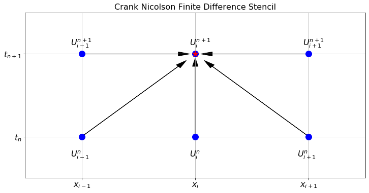
Exercise 6.45 To graphically show the Crank Nicolson method we can again use a finite difference stencil to show where the information is coming from and where it is going to. In Figure 6.10 notice that there are three points at the new time step that are used to calculate the value of $U_i^{n+1}$ at the new time step. Sketch a similar image for the original implicit scheme from Exercise 6.43

Figure 6.10: The finite difference stencil for the Crank Nicolson method.

6.6 The Wave Equation

The problems that we’ve dealt with thus far all model natural diffusion processes: heat transport, molecular diffusion, etc. Another interesting physical phenomenon is that of wave propagation. Previously it was given that the 1D wave equation is \[\begin{aligned} u_{tt} = c u_{xx} \label{eqn:wave1D} \end{aligned}\] where $c$ is a parameter modeling the stiffness of the medium the wave is traveling through. With homogeneous Dirichlet boundary conditions we can think of this as the behavior of a guitar string after it has been plucked. If the boundaries are in motion then the model might be of someone wiggling a taught string from one end.

So far we have just accepted that this is the wave equation, but we should pause now and look at where the equation comes from. We will stick with 1 spatial dimension and imagine that we are modeling the displacement of a plucked guitar string. Let $u(t,x)$ be the displacement of the string from equilibrium. From Newton’s second law we know that $F = ma$ where the force here is the tension in the string. From Calculus, the acceleration is the second time derivative of the displacement. Hence, for a string of density $\rho$ over length $\Delta x$ we have \[ma = \rho \Delta x \frac{\partial^2 u}{\partial t^2}\] and we now have the equation \[\text{tension in the string} = \rho \Delta x \frac{\partial^2 u}{\partial t^2}.\]

If we assume that there is no bending or side-to-side motion of the spring, the tension vector must be tangential to the string. It would be good to draw a picture now:

Draw a curve representing the string.
Pick two points on the curve representing the left and right side of an interval of length $\Delta x$.
Draw a vector tangent to the string at the left point. The angle from horizontal will be called $\theta_{\text{left}}$
Draw a vector tangent to the string at the right point. The angle from horizontal will be called $\theta_{\text{right}}$

If we are interested in a segment of string of length $\Delta x$ then the vertical motion will be dictated by the difference between the vertical components of the tensions at the two endpoints \[\text{tension in the spring} = T_{\text{right}} \sin \theta_{\text{right}} - T_{\text{left}} \sin \theta_{\text{left}}\] Since the motion is only vertical we must have that the horizontal tensions are equal and constant \[T_{\text{right}} \cos \theta_{\text{right}} = T_{\text{left}} \cos \theta_{\text{left}} = T.\]

If we divide both sides of the equation \[T_{\text{right}} \sin \theta_{\text{right}} - T_{\text{left}} \sin \theta_{\text{left}} = \rho \Delta x \frac{\partial^2 u}{\partial t^2}\] by the constant tension $T$ we get \[\tan\theta_{\text{right}} - \tan\theta_{\text{left}} = \frac{\rho \Delta x}{T} \frac{\partial^2 u}{\partial t^2}.\] Recognizing that the tangent of the angle will just be the slopes at the right and left points we now have \[u_x(t,x+\Delta x) - u_x(t,x) = \frac{\rho \Delta x}{T} \frac{\partial^2 u}{\partial t^2}\] which can be rearranged to \[\frac{T}{\rho} \frac{u_x(t,x+\Delta x) - u_x(t,x)}{\Delta x} = \frac{\partial^2 u}{\partial t^2}.\]

Allowing $\Delta x$ to get arbitarily small the difference quotient on the left-hand side becomes the second spatial derivative and we arrive at the 1D wave equation \[\frac{\partial^2 u}{\partial t^2} = c \frac{\partial^2 u}{\partial x^2}\] where we have defined $c = T/\rho$ as a parameter describing the stiffness of the string. The 2D and 3D derivations are similar but a bit trickier with the trig and geometry.

For the remainder of this section we will focus on approximating solutions to the wave equation in 1D, 2D, and 3D numerically.

Exercise 6.46 Let’s write code to numerically solve the 1D wave equation. As before, we use the notation $U_i^n$ to represent the approximate solution $u(t,x)$ at the point $t=t_n$ and $x=x_i$.

Give a reasonable discretization of the second derivative in time: \[ u_{tt}(t_{n}, x_i) \approx \underline{\hspace{1in}}. \]
Give a reasonable discretization of the second derivative in space: \[ u_{xx}(t_n, x_i) \approx \underline{\hspace{1in}}. \]
Put your answers to parts (a) and (b) together with the wave equation to get \[ \frac{??? - ??? + ???}{\Delta t^2} = c \frac{??? - ??? + ???}{\Delta x^2}. \]
Solve the equation from part (c) for $U_i^{n+1}$. The resulting difference equation is the finite difference scheme for the 1D wave equation.
You should notice that the finite difference scheme for the wave equation references two different times: $U_i^n$ and $U_i^{n-1}$. Based on this observation, what information do we need to in order to actually start our numerical solution?
Consider the wave equation $u_{tt} = 2 u_{xx}$ in $x \in (0,1)$ with $u(0,x) = 4x(1-x)$, $u_t(0,x) = 0$, and $u(t,0) = u(t,1) = 0$. Use the finite difference scheme that you built in this problem to approximate the solution to this PDE.

Figure 6.11 shows the finite difference stencil for the 1D wave equation. Notice that we need two prior time steps in order to advance to the new time step. This means that in order to start the finite difference scheme for the wave equation we need to have information about time $t_0$ and also time $t_1$. We get this information by using the two initial conditions $u(0,x)$ and $u_t(0,x)$.

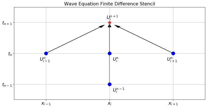
Figure 6.11: The finite difference stencil for the 1D wave equation.

Exercise 6.47 The ratio $c\Delta t^2 / \Delta x^2$ shows up explicitly in the finite difference scheme for the 1D wave equation. Just like in the heat equation, this parameter controlls when the finite difference solution will be stable. Experiment with your finite difference solution and conjecture a value of $a = c \Delta t^2 / \Delta x^2$ which divides the regions of stability versus instability. Your answer should be in the form:

If $a = c\Delta t^2 / \Delta x^2 < \underline{\hspace{0.5in}}$ then the finite difference scheme for the 1D wave equation will be stable. Otherwise it will be unstable.

Exercise 6.48 Show several plots demonstrating what occurs to the finite difference solution of the wave equation when the parameters are in the unstable region and right on the edge of the unstable region.

Exercise 6.49 What is the expected error in the finite difference scheme for the 1D wave equation? What does this mean in plain English?

Exercise 6.50 Use your finite difference code to solve the 1D wave equation \[ u_{tt} = c u_{xx} \] with boundary conditions $u(t,0) = u(t,1) = 0$, initial condition $u(0,x) = 4x(1-x)$, and zero initial velocity. Experiment with different values of $c$. What does the parameter $c$ to the wave? Give a physical interpretation of $c$.

Exercise 6.51 Solve the 1D wave equation \[ u_{tt} = u_{xx} \] with Dirichlet boundary conditions $u(t,0) = 0.4 \sin(\pi t)$ and $u(t,1) = 0$ along with initial condition $u(0,x) = 0$ and zero initial velocity. This time the left-hand boundary is being controlled externally and the string starts off at equilibrium. Give a physical situation where this sort of setup might arise. Then modify your solution so that both sides of the string are being wiggled at different frequencies.

Exercise 6.52 Now consider the 2D wave equation \[ u_{tt} = c\left( u_{xx} + u_{yy} \right). \] We want to build a numerical solution to this new PDE. Just like with the 2D heat equation we propose the notation $U_{i,j}^n$ for the approximation of the function $u(t,x,y)$ at the point $t=t_n$, $x=x_i$, and $y=y_j$.

Give discretizations of the derivatives $u_{tt}$, $u_{xx}$, and $u_{yy}$.
Substitute your discretizations into the 2D wave equation, make the simplifying assumption that $\Delta x = \Delta y$, and solve for $U_{i,j}^{n+1}$. This is the finite difference scheme for the 2D wave equation.
Write code to implement the finite difference scheme from part (b) on the domain $(x,y) \in (0,1)\times (0,1)$ with homogeneous Dirichlet boundary conditions, initial condition $u(0,x,y) = \sin(2\pi (x-0.5))\sin(2\pi(y-0.5))$, and zero initial velocity.
Draw the finite difference stencil for the 2D heat equation.

Exercise 6.53 What is the region of stability for the finite difference scheme on the 2D wave equation? Produce several plots showing what happens when we are in the unstable region as well as when we are right on the edge of the stable region.

Exercise 6.54 Solve the 2D wave equation on the unit square with $u$ starting at rest and being driven by a wave coming in from one boundary.

6.7 Traveling Waves

Now we turn our attention to a new PDE: the traveling wave equation \[ u_t + v u_x = 0. \] In this equation $u(t,x)$ is the height of a wave at time $t$ and spatial location $x$. The parameter $v$ is the velocity of the wave. Imagine this as sending a single solitary wave pulsing down a taught rope or as sending a single pulse of light down a fiber optic cable.

Exercise 6.55 Consider the PDE $u_t + v u_x = 0$. There is a very easy way to get an analytic solution to this traveling wave equation. If we have the initial condition $u(0,x) = f(x) = e^{-(x-4)^2}$ then we claim that $u(t,x) = f(x-vt)$ is an analytic solution to the PDE. More explicitely, we are claiming that \[ u(t,x) = e^{-(x-vt-4)^2} \] is the analytic solution to the PDE. Let’s prove this.

Take the $t$ derivative of $u(t,x)$.
Take the $x$ derivative of $u(t,x)$.
The PDE claims that $u_t + vu_x = 0$. Verify that this equal sign is indeed true.

Exercise 6.56 Now we would like to visualize the solution to the PDE from the previous exercise. The Python code below gives an interactive visual of the solution. Experiment with different values of $v$ and different initial conditions.

import numpy as np
import matplotlib.pyplot as plt
from matplotlib import animation, rc
from IPython.display import HTML

v = 1
f = lambda x: np.exp(-(x-4)**2)
u = lambda t, x: f(x - v*t)
x = np.linspace(0,10,100)
t = np.linspace(0,10,100)

fig, ax = plt.subplots()
plt.close()
ax.grid()
ax.set_xlabel('x')
ax.set_xlim(( 0, 10))
ax.set_ylim(( -0.1, 1))
frame, = ax.plot([], [], linewidth=2, linestyle='--')

def animator(N):
  ax.set_title('Time='+str(t[N]))
  frame.set_data(x,???) # plot the correct time step for u(t,x)
  return (frame,)

PlotFrames = range(0,len(t),1) 
anim = animation.FuncAnimation(fig, 
                               animator, 
                               frames=PlotFrames, 
                               interval=100, 
                              )

rc('animation', html='jshtml') # embed in the HTML for Google Colab
anim

Theorem 6.6 If $u_t + v u_{x} = 0$ with initial condition $u(0,x) = f(x)$ then the function $u(t,x) = f(x-vt)$ is an analytic solution to the PDE.

Exercise 6.57 Use the chain rule to prove the previous theorem.

The traveling wave equation $u_t + vu_x = 0$ has a very nice analytic solution which we can always find. Therefore there is no need to ever find a numerical solution – we can just write down the analytic solution if we are given the initial condition. As it turns out though the numerical solutions exhibit some very interesting behavior.

Exercise 6.58 Consider the traveling wave equation $u_t + vu_x = 0$ with initial condition $u(0,x) = f(x)$ for some given function $f$ and boundary condition $u(t,0) = 0$. To build a numerical solution we will again adopt the notation $U_i^n$ for the approximation to $u(t,x)$ at the point $t=t_n$ and $x=x_i$.

Write an approximation of $u_t$ using $U_i^{n+1}$ and $U_i^n$.
Write an approximation of $u_x$ using $U_{i+1}^n$ and $U_i^n$.
Substitute your answers from parts (a) and (b) into the traveling wave equation and solve for $U_i^{n+1}$. This is our first finite difference scheme for the traveling wave equation.
Write Python code to get the finite difference approximation of the solution to the PDE. Plot your finite difference solution on top of the analytic solution for $f(x) = e^{-(x-4)^2}$. What do you notice? Can you stabilize this method by changing the values of $\Delta t$ and $\Delta x$ like with did with the heat and wave equations?

The finite difference scheme that you built in the previous exercise is called the downwind scheme for the traveling wave equation. Figure 6.12 shows the finite difference stencil for this scheme. We call this scheme “downwind” since we expect the wave to travel from left to right and we can think of a fictitious wind blowing the solution from left to right. Notice that we are using information from “downwind” of the point at the new time step.

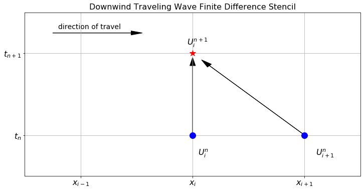
Figure 6.12: The finite difference stencil for the 1D downwind scheme on the traveling wave equation.

Exercise 6.59 You should have noticed in the previous exercise that you cannot reasonbly stabilize the finite difference scheme. Propose several reasons why this method appears to be unstable no matter what you use for the ratio $v \Delta t / \Delta x$.

Exercise 6.60 One of the troubles with the finite difference scheme that we have built for the traveling wave equation is that we are using the information at our present spatial location and the next spatial location to the right to propogate the solution forward in time. The trouble here is that the wave is moving from left to right, so the interesting information about the next time step’s solution is actually coming from the left, not the right. We call this “looking upwind” since you can think of a fictitious wind blowing from left to right, and we need to look “upwind” to see what is coming at us. If we write the spatial derivative as \[ u_x \approx \frac{U_i^n - U_{i-1}^n}{\Delta x} \] we still have a first-order approximation of the derivative but we are now looking left instead of right for our spatial derivative. Make this modification in your finite difference code for the traveling wave equation (call it the “upwind method”). Approximate the solution to the same PDE as we worked with in the previous exercises. What do you notice now?

Figure 6.13 shows the finite difference stencil for the upwind scheme. We call this scheme “up” since we expect the wave to travel from left to right and we can think of a fictitious wind blowing the solution from left to right. Notice that we are using information from “upwind” of the point at the new time step.

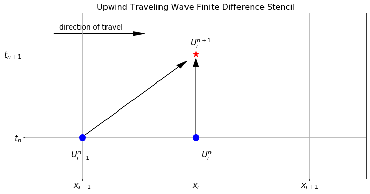
Figure 6.13: The finite difference stencil for the 1D downwind scheme on the traveling wave equation.

Exercise 6.61 Complete the following sentences:

In the downwind finite difference scheme for the traveling wave equation, the approximate solution moves at the correct speed, but …
In the upwind finite difference scheme for the traveling wave equation, the approximate solution moves at the correct speed, but …

Exercise 6.62 Neither the downwind nor the upwind solutions for the traveling wave equation are satisfactory. They completely miss the interesting dynamics of the analytic solution to the PDE. Some ideas for stabilizing the finite difference solution for the traveling wave equation are as follows. Implement each of these ideas and discuss pros and cons of each. Also draw a finite difference stencil for each of these methods.

Perhaps one of the issues is that we are using first-order methods to approximate $u_t$ and $u_x$. What if we used a second-order approximation for these first derivatives \[ u_t \approx \frac{U_i^{n+1} - U_i^{n-1}}{2\Delta t} \quad \text{ and } \quad u_x \approx \frac{U_{i+1}^n - U_{i-1}^n}{2\Delta x}? \] Solve for $U_i^{n+1}$ and implement this method. This is called the leapfrog method.
For this next method let’s stick with the second-order approximation of $u_x$ but we’ll do something clever for $u_t$. For the time derivative we originally used \[ u_t \approx \frac{U_i^{n+1} - U_i^n}{\Delta t} \] what happens if we replace $U_i^n$ with the average value from the two surrounding spatial points \[ U_i^n \approx \frac{1}{2} \left( U_{i+1}^n + U_{i-1}^n \right)? \] This would make our approximation of the time derivative \[ u_t \approx \frac{U_i^{n+1} - \frac{1}{2} \left( U_{i+1}^n + U_{i-1}^n \right)}{\Delta t}. \] Solve this modified finite difference equation for $U_i^{n+1}$ and implement this method. This is called the Lax-Friedrichs method.
Finally we’ll do something very clever (and very counter intuitive). What if we inserted some artificial diffusion into the problem? You know from your work with the heat equation that diffusion spreads a solution out. The downwind scheme seemed to have the issue that it was bunching up at the beginning and end of the wave, so artificial diffusion might smooth this out. The Lax-Wendroff method does exactly that: take a regular Euler-type step in time \[ u_t \approx \frac{U_i^{n+1} - U_i^n}{\Delta t}, \] use a second-order centered difference scheme in space to approximate $u_x$ \[ u_x \approx \frac{U_{i+1}^n - U_{i-1}^n}{2\Delta x}, \] but add on the term \[ \left( \frac{v^2 \Delta t^2}{2\Delta x^2} \right) \left( U_{i-1}^n - 2 U_i^n + U_{i+1}^n \right) \] to the right-hand side of the equation. Notice that this new term is a scalar multiple of the second-order approximation of the second derivative $u_{xx}$. Solve this equation for $U_i^{n+1}$ and implement the Lax-Wendroff method.

6.8 The Laplace and Poisson Equations

Exercise 6.63 Consider the 1D heat equation $u_t = 1 u_{xx}$ with boundary conditions $u(t,0) = 0$ and $u(t,1)=1$ and initial condition $u(0,x) = 0$.

Describe the physical setup for this problem.
Recall that the solution to a differential equation reaches a steady state (or equilibrium) when the time rate of change is zero. Based on the physical system, what is the steady state heat profile for this PDE?
Use your 1D heat equation code to show the full time evolution of this PDE. Run the simulation long enough so that you see the steady state heat profile.

Exercise 6.64 Now consider the forced 1D heat equation $u_t = u_{xx} + e^{-(x-0.5)^2}$ with the same boundary and initial conditions as the previous exercise. The exponential forcing function introduced in this equation is an external source of heat (like a flame held to the middle of the metal rod).

Conjecture what the steady state heat profile will look like for this particular setup. Be able to defend your answer.
Modify your 1D heat equation code to show the full time evolution of this PDE. Run the simulation long enough so that you see the steady state heat profile.

Exercise 6.65 Next we’ll examine 2D steady state heat profiles. Consider the PDE $u_t = u_{xx} + u_{yy}$ with boundary conditions $u(t,0,y) = u(t,x,0) = u(t,x,1) = 0$ and $u(t,1,y) = 1$ with initial condition $u(0,x,y) = 0$.

Describe the physical setup for this problem.
Based on the physical system, describe the steady state heat profile for this PDE. Be sure that your steady state solution still satisfies the boundary conditions.
Use your 2D heat equation code to show the full time evolution of this PDE. Run the simulation long enough so that you see the steady state heat profile.

Exercise 6.66 Now consider the forced 2D heat equation $u_t = u_{xx} + u_{yy} + 10e^{-(x-0.5)^2-(y-0.5)^2}$ with the same boundary and initial conditions as the previous exercise. The exponential forcing function introduced in this equation is an external source of heat (like a flame held to the middle of the metal sheet).

Conjecture what the steady state heat profile will look like for this particular setup. Be able to defend your answer.
Modify your 2D heat equation code to show the full time evolution of this PDE. Run the simulation long enough so that you see the steady state heat profile.

Up to this point we have studied PDEs that all depend on time. In many applications, however, we are not interested in the transient (time dependent) behavior of a system. Instead we are often interested in the steady state solution when the forces in question are in static equilibrium. Two very famous time-independent PDEs are the Laplace Equation \[ u_{xx} + u_{yy} + u_{zz} = 0 \] and the Poisson equation \[ u_{xx} + u_{yy} + u_{zz} = f(x,y,z). \] Notice that both the Laplace and Poisson equations are the equations that we get when we consider the limit $u_t \to 0$. In the limit when the time rate of change goes to zero we are actually just looking at the eventual steady state heat profile resulting from the initial and boundary conditions of the heat equation. In the previous exercises you already wrote code that will show the steady state profiles in a few setups. The trouble with the approach of letting the time-dependent simulation run for a long time is that the finite difference solution for the heat equation is known to have stability issues. Moreover, it may take a lot of computational time for the solution to reach the eventual steady state. In the remainder of this section we look at methods of solving for the steady state directly – without examining any of the transient behavior. We will first examine a 1D version of the Laplace and Poisson equations.

Exercise 6.67 Consider a 1-dimensional rod that is infinitely thin and has unit length. For the sake of simplicity assume the following:

the specific heat of the rod is exactly 1 for the entire length of the rod,
the temperature of the left end is held fixed at $u(0) = 0$,
the temperature of the right end is held fixed at $u(1) = 1$, and
the temperature has reached a steady state.

You can assume that the temperatures are reference temperatures instead of absolute temperatures, so a temperature of “0” might represent room temperature.

Since there are no external sources of heat we model the steady-state heat profile we must have $u_t = 0$ in the heat equation. Thus the heat equation collapses to $u_{xx} = 0$. This is exactly the one dimensional Laplace equation.

To get an exact solution of the Laplace equation in this situation we simply need to integrate twice. Do the integration and write the analytic solution (there should be no surprises here).
To get a numerical solution we first need to partition the domain into finitely many point. For the sake of simplicity let’s say that we subdivide the interval into 5 equal sub intervals (so there are 6 points including the endpoints). Furthermore, we know that we can approximate $u_{xx}$ as \[ u_{xx} \approx \frac{U_{i+1} - 2U_i + U_{i-1}}{\Delta x^2}. \] Thus we have 6 linear equations: \[\begin{aligned} U_0 &= 1 \quad \text{(left boundary condition)}\\ \frac{U_2 - 2U_1 + U_0}{\Delta x^2} &= 0 \\ \frac{U_3 - 2U_2 + U_1}{\Delta x^2} &= 0 \\ \frac{U_4 - 2U_3 + U_2}{\Delta x^2} &= 0 \\ \frac{U_5 - 2U_4 + U_3}{\Delta x^2} &= 0 \\ U_5 &= 0 \quad \text{(right boundary condition).} \end{aligned}\] Notice that there are really only four unknowns since the boundary conditions dictate two of the temperature values. Rearrange this system of equations into a matrix equation and solve for the unknowns $U_1$, $U_2$, $U_3$, and $U_4$. Your coefficient matrix should be $4 \times 4$.
Compare your answers from parts (a) and (b).
Write code to build the numerical solution with an arbitrary value for $\Delta x$ (i.e. an arbitrary number of sub intervals). You should build the linear system automatically in your code.

Exercise 6.68 Solve the 1D Laplace equation with Dirichlet boundary conditions is rather uninteresting since the answer will alway be a linear function connecting the two boundary conditions. Prove this.

The Poisson equation, $u_{xx} = f(x)$, is more interesting than the Laplace equation in 1D. The function $f(x)$ is called a forcing function. You can think of it this way: if $u$ is the amount of force on a linear bridge, then $f$ might be a function that gives the distribution of the forces on the bridge due to the cars sitting on the bridge. In terms of heat we can think of this as an external source of heat energy warming up the one-dimensional rod somewhere in the middle (like a flame being held to one place on the rod).

Exercise 6.69 How would we analytically solve the Poisson equation $u_{xx} = f(x)$ in one spatial dimension? As a sample problem consider $x\in [0,1]$, the forcing function $f(x) = 5\sin(2 \pi x)$ and boundary conditions $u(0) = 2$ and $u(1) = 0.5$. Of course you need to check your answer by taking two derivatives and making sure that the second derivative exactly matches $f(x)$. Also be sure that your solution matches the boundary conditions exactly.

Exercise 6.70 Now we can solve the Poisson equation from the previous problem numerically. Let’s again build this with a partition that contains only 6 points just like we did with the Laplace equation a few exercise ago. We know the approximation for $u_{xx}$ so we have the linear system \[\begin{aligned} U_0 &= 2 \quad \text{(left boundary condition)}\\ \frac{U_2 - 2U_1 + U_0}{\Delta x^2} &= f(x_1) \\ \frac{U_3 - 2U_2 + U_1}{\Delta x^2} &= f(x_2) \\ \frac{U_4 - 2U_3 + U_2}{\Delta x^2} &= f(x_3) \\ \frac{U_5 - 2U_4 + U_3}{\Delta x^2} &= f(x_4) \\ U_5 &= 0.5 \quad \text{(right boundary condition).} \end{aligned}\]

Rearrange the system of equations as a matrix equation and then solve the system for $U_1, U_2, U_3$, and $U_4$. There are really only four equations so your matrix should be $4 \times 4$.
Compare your solution from part (a) to the function values that you found in the previous exercise.
Now generalize the process of solving the 1D Poisson equation for an arbitrary value of $\Delta x$. You will need to build the matrix and the right-hand side in your code. Test your code on new forcing functions and new boundary conditions.

Exercise 6.71 The previous exercises only account for Dirichlet boundary conditions (fixed boundary conditions). We would now like to modify our Poisson solution to allow for a Neumann condition: where we know the derivative of $u$ at one of the boundaries. The statement of the problem is as follows: \[\text{Solve: } u_{xx} = f(x) \quad \text{on} \quad x \in (0,1) \quad \text{with} \quad u_x(0) = \alpha \quad \text{and} \quad u(1) = \beta.\] The derivative condition on the boundary can be approximated by using a first-order approximation of the derivative, and as a consequence we have one new equation. Specifically, if we know that $u_x(0) = \alpha$ then we can approximate this condition as \[ \frac{U_1 - U_0}{\Delta x} = \alpha, \] and we simply need to add this equation to the system that we were solving in the previous exercise. If we go back to our example of a partition with 6 points the system becomes \[\begin{aligned} \frac{U_1 - U_0}{\Delta x} &= \alpha \quad \text{(left boundary condition)}\\ \frac{U_2 - 2U_1 + U_0}{\Delta x^2} &= f(x_1) \\ \frac{U_3 - 2U_2 + U_1}{\Delta x^2} &= f(x_2) \\ \frac{U_4 - 2U_3 + U_2}{\Delta x^2} &= f(x_3) \\ \frac{U_5 - 2U_4 + U_3}{\Delta x^2} &= f(x_4) \\ U_5 &= \beta \quad \text{(right boundary condition).} \end{aligned}\] There are 5 equations this time.

With a 6 point grid solve the Poisson equation $u_{xx} = 5\sin(2\pi x)$ with $u_x(0) = 0$ and $u(1) = 3$.
Modify your code from part (a) to solve the same problem but with a much smaller value of $\Delta x$. You will need to build the matrix equation in your code.

Exercise 6.72 (The 2D Poisson Equation) We conclude this section, and chapter, by examining the two dimensional Poisson equations. As a sample problem, we want to solve the Poisson equation $u_{xx} + u_{yy} = f(x,y)$ on the domain $(x,y) \in (0,1)\times (0,1)$ with homogenous Dirichlet boundary conditions and focing function $f(x,y) = -20\text{exp}\left( -\frac{(x-0.5)^2 + (y-0.5)^2}{0.05} \right)$ numerically. We are going to start with a $6 \times 6$ grid of points and explicitly write down all of the equations. In Figure 6.14 the red stars represent boundary points where the value of $u(x,y)$ is known and the blue interior points are the ones where $u(x,y)$ is yet unknown. It should be clear that we should have two indices for each point (one for the $x$ position and one for the $y$ position), but it should also be clear that this will cause problems when writing down the resulting system of equations as a matrix equation (stop and think carefully about this). Therefore, in Figure 6.14 we propose an index, $k$, starting at the top left of the uninown nodes and reading left to right (just like we do with Python arrays).

Start by discretizing the 2D Poisson equation $u_{xx} + u_{yy} = f(x,y)$. For simplicity we assume that $\Delta x = \Delta y$ so that we can combine like terms from the $x$ derivative and the $y$ derivative. Fill in the missing coefficients and indices below. \[U_{i+1,j} + U_{i,j-1} - (\underline{\hspace{0.2in}}) U_{\underline{\hspace{0.2in}},\underline{\hspace{0.2in}}} + U_{\underline{\hspace{0.2in}},\underline{\hspace{0.2in}}} + U_{\underline{\hspace{0.2in}},\underline{\hspace{0.2in}}} = \Delta x^2 f(x_i,y_i)\]
In Figure 6.14 we see that there are 16 total equations resulting from the discretization of the Poisson equation. Your first task is to write all 16 of these equations. We’ll get you started:

\[\begin{aligned} \text{$k=0$: } &\quad U_{k=1} + {\color{red} U_{i=1,j=0} } - 4U_{k=0} + {\color{red} U_{i=0,j=1} } + U_{k=4} = \Delta x^2 f(x_1,y_1) \\ \text{$k=1$: } &\quad U_{k=2} + U_{k=0} - 4U_{k=1} + {\color{red} U_{i=0,j=2} } + U_{k=5} = \Delta x^2 f(x_1,y_2) \\ & \qquad \vdots \\ \text{$k=15$: } &\quad {\color{red} U_{i=4,j=5}} + U_{k=14} - 4 U_{k=15} + U_{k=11} + {\color{red} U_{i=5,j=4}} = \Delta x^2 f(x_4,y_4) \end{aligned}\]

In this particular example we have homogeneous Dirichlet boundary conditions so all of the boundary values are zero. If this was not the case then every boundary value would need to be moved to the right-hand sides of the equations. c. We now have a $16 \times 16$ matrix equation to write based on the equations from part (b). Each row and column of the matrix equation is indexed by $k$. The coefficient matrix $A$ is started for you below. Write the whole thing out and fill in the blanks. Notice that this matrix has a much more complicated structure than the coefficient matrix in the 1D Poisson and Laplace equations.

\[A = \begin{pmatrix} -4 & 1 & 0 & 0 & 1 & 0 & 0 & 0 & \cdots & 0 \\ 1 & -4 & 1 & 0 & 0 & 1 & 0 & 0 & \cdots & 0 \\ 0 & 1 & -4 & 1 & 0 & 0 & 1 & 0 & \cdots & 0 \\ 0 & 0 & 1 & -4 & 1 & 0 & 0 & 1 & & \\ 1 & 0 & 0 & 0 & -4 & 1 & 0 & 0 & \ddots & \\ 0 & & & & & & & & & \\ \vdots & & & & & & & & & \\ & & & & & & & & & \\ & & & & & & & & & -4 \\ \end{pmatrix}\]

In the coefficient matrix from part (c) notice that the small matrix \[\begin{pmatrix} -4 & 1 & 0 & 0 \\ 1 & -4 & 1 & 0 \\ 0 & 1 & -4 & 1 \\ 0 & 0 & 1 & -4 \end{pmatrix}\] shows up in blocks along the main diagonal. If you have a hard copy of the matrix go back and draw a box around these blocks in the coefficient matrix. Also notice that there are diagonal bands of $1^s$. Discuss the following:
1. Why are the blocks $4 \times 4$?
2. How could you have predicted the location of the diagonal bands of $1^s$?
3. What would the structure of the matrix look like if we partitioned the domain into a $10 \times 10$ grid of points instead of a $6 \times 6$ grid (including the boundary points)?
4. Why is it helpful to notice this structure?
The right-hand side of the matrix equation resulting the your system of equations from part (b) is \[\boldsymbol{b} = \Delta x^2 \begin{pmatrix} f(x_1,y_1) \\ f(x_1,y_2) \\ f(x_1,y_3) \\ f(x_1,y_4) \\ f(x_2,y_1) \\ f(x_2,y_2) \\ \vdots \\ \\ f(x_4,y_y) \end{pmatrix}.\] Notice the structure of this vector. Why is it structured this way? Why is it useful to notice this?
Write Python code to solve the problem at hand. Recall that $f(x,y) = -20\exp\left(-\frac{-(x-0.5)^2+(y-0.5)^2}{0.05}\right)$. Show a contour plot of your solution. This will take a little work changing the indices back from $k$ to $i$ and $j$. Think carefully about how you want to code this before you put fingers to keyboard. You might want to use the np.block() command to build the coefficient matrix efficiently or you can use loops with carefully chosen indices.
(Challenge) Generalize your code to solve the Poisson equation with a much smaller value of $\Delta x = \Delta y$.
One more significant observation should be made about the 2D Poisson equation on this square domain. Notice that the corner points of the domain (e.g. $i=0, j=0$ or $i=5, j=0$) are never included in the system of equations. What does this mean about trying to enforce boundary conditions that only apply at the corners?

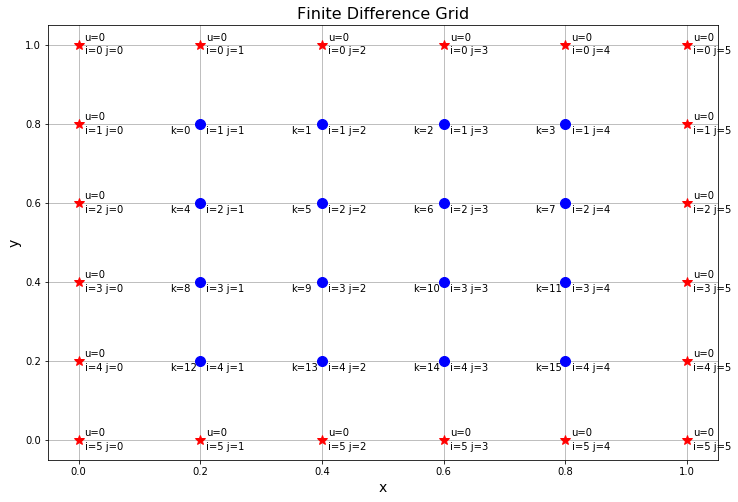
Figure 6.14: A finite difference grid for the Poisson equation with 6 grid points in each direction.

6.9 Exercises

6.9.1 Algorithm Summaries

Exercise 6.73 Explain in clear language what it means to check an analytic solution to a differential equation.

Exercise 6.74 Explain in clear language what Dirichlet boundary conditions are.

Exercise 6.75 Explain in clear language what Neumann boundary conditions are.

Exercise 6.76 Show the full mathematical details for building a first-order in time and second-order in space approximation method for the one-dimensional heat equation. Explain what the order of the error means in this context

Exercise 6.77 Show the full mathematical details for building a second-order in time and second-order in space approximation method for the one-dimensional wave equation. Explain what the order of the error means in this context

Exercise 6.78 Show the full mathematical details for building a first-order in time and second-order in space approximation method for the two-dimensional heat equation. Explain what the order of the error means in this context

Exercise 6.79 Show the full mathematical details for building a second-order in time and second-order in space approximation method for the two-dimensional wave equation. Explain what the order of the error means in this context

Exercise 6.80 Explain in clear language what it means for a finite difference method to be stable vs unstable.

Exercise 6.81 Show the full mathematical details for solving the 1D heat equation using the implicit and Crank-Nicolson methods.

Exercise 6.82 Show the full mathematical details for building a downwind finite difference scheme for the traveling wave equation. Discuss the primary disadvantages of the downwind scheme.

Exercise 6.83 Show the full mathematical details for building an upwind finite difference scheme for the traveling wave equation. Discuss the primary disadvantages of the upwind scheme.

Exercise 6.84 Show the full mathematical details for numerically solving the 1D Laplace and Poisson equations.

6.9.2 Applying What You’ve Learned

Exercise 6.85 In this problem we will solve a more realistic 1D heat equation. We will allow the diffusivity to change spatially, so $D = D(x)$ and we want to solve \[u_t = \left( D(x) u_x \right)_x\] on $x \in (0,1)$ with Dirichlet boundary conditions $u(t,0) = u(t,1) = 0$ and initial condition $u(0,x) = \sin(2 \pi x)$. This is “more realistic” since it would be rare to have a perfectly homogenous medium, and the function $D$ reflects any heterogeneities in the way the diffusion occurs. In this problem we will take $D(x)$ to be the parabola $D(x)= x^3(1-x)$. We start by doing some calculus to rewrite the differential equation: \[u_t = D(x) u_{xx}(x) + D'(x) u_x(x).\]

Your jobs are:

Describe what this choice of $D(x)$ might mean physically in the heat equation.
Write an explicit scheme to solve this problem by using centered differences for the spatial derivatives and an Euler-type discretization for the temporal derivative. Write a clear and thorough explanation for how you are doing the discretization as well as a discussion for the errors that are being made with each discretization.
Write a script to find an approximate solution to this problem.
Write a clear and thorough discussion about how your will choose $\Delta x$ and $\Delta t$ to give stable solutions to this equation.
Graphically compare your solution to this problem with a heat equation where $D$ is taken to be the constant average diffusivity found by calculating $D_{ave} = \int_0^1 D(x) dx.$ How does the changing diffusivity change the shape of the solution?

Exercise 6.86 In a square domain create a function $u(0,x,y)$ that looks like your college logo. The simplest way to do this might be to take a photo of the logo, crop it to a square, and use the scipy.ndimage.imread command to read in the image. Use this function as the initial condition for the heat equation on a square domain with homogeneous Dirichlet boundary conditions. Numerically solve the heat equation and show an animation for what happens to the logo as time evolves.

Exercise 6.87 Repeat the previous exercise but this time solve the wave equation with the logo as the initial condition.

Exercise 6.88 The explicit finite difference scheme that we built for the 1D heat equation in this chapter has error on the order of $\mathcal{O}(\Delta t) + \mathcal{O}(\Delta x^2)$. Explain clearly what this means. Then devise a numerical experiment to empirically test this fact. Clearly explain your thought process and show sufficient plots and mathematics to support your work.

Exercise 6.89 Suppose that we have a concrete slab that is 10 meters in length, with the left boundary held at a temperature of $75^\circ$ and the right boundary held at a temperature of $90^\circ$. Assume that the thermal diffusivity of concrete is about $k = 10^{-5}$ m$^2$/s. Assume that the initial temperature of the slab is given by the function $T(x) = 75 + 1.5x - 20 \sin( \pi x / 10)$. In this case, the temperature can be analytically solved by the function $T(t,x) = 75 + 1.5x - 20 \sin(\pi x / 10) e^{-ct}$ for some value of $c$.

Working by hand (no computers!) test the proposed analytic solution by substituting it into the 1D heat equation and verifying that it is indeed a solution. In doing so you will be able to find the correct value of $c$.
Write numerical code to solve this 1D heat equation. The output of your code should be an animation showing how the error between the numerical solution and the analytic solution evolve in time.

Exercise 6.90 (This problem is modified from [11]. The data given below is real experimental data provided courtesy of the authors.)

Harry and Sally set up an experiment to gather data specifically for the heat diffusion through a long thin metal rod. Their experimental setup was as follows.

The ends of the rod are submerged in water baths at different temperatures and the heat from the hot water bath (on the right hand side) travels through the metal to the cooler end (on the left hand side).
The temperature of the rod is measured at four locations; those measurements are sent to a Raspberry Pi, which processes the raw data and sends the collated data to be displayed on the computer screen.
They used a metal rod of length $L = 300 mm$ and square cross-sectional width $3.2 mm$.
The temperature sensors were placed at $x_1 = 47mm$, $x_2 = 94mm$, $x_3 = 141mm$, and $x_4 = 188mm$ as measured from the cool end (the left end).
Foam tubing, with a thickness of 25 mm, was wrapped around the rod and sensors to provide some insulation.
The ambient temperature in the room was $22^\circ C$ and the cool water bath is a large enough reservoir that the left side of the rod is kept at $22^\circ C$.

The data table below gives temperature measurements at 60 second intervals for each of the four sensors.

Time (sec)	Sensor 188	Sensor 141	Sensor 94	Sensor 47
0	22.8	22	22	22
60	29.3	24.4	23.2	22.8
120	35.7	27.5	25.9	25.2
180	41.8	30.3	27.9	26.8
240	45.8	33.8	30.6	29.2
300	48.2	36.5	32.6	31.2
360	50.6	37.7	34.2	32
420	53.4	38.5	34.9	32.8
480	53	38.9	35.3	33.6
540	53	40.4	36.5	34.8
600	55.1	41.2	37.3	35.2
660	54.7	42	38.1	35.6
720	54.7	42.4	38.1	36
780	54.7	42.4	38.1	36.4
840	54.7	42	38.5	36
900	57.5	41.2	37.7	35.6
960	56.3	40.8	37.3	35.6

At time time $t=960$ seconds the temperatures of the rod are essentially at a steady state. Use this data to make a prediction of the temperature of the hot water bath located at $x=300mm$.
The thermal diffusivity, $D$, of the metal is unknown. Use your numerical solution in conjunction with the data to approximate the value of $D$. Be sure to fully defend your process.
It is unlikely that your numerical solution to the heat equation and the data from part (b) match very well. What are some sources of error in the data or in the heat equation model?

You can load the data directly with the following code.

import numpy as np
import pandas as pd
URL1 = 'https://raw.githubusercontent.com/NumericalMethodsSullivan'
URL2 = '/NumericalMethodsSullivan.github.io/master/data/'
URL = URL1+URL2
data = np.array( pd.read_csv(URL+'Exercise6_1dheatdata.csv') )
# Exercise6_1dheatdata.csv

Exercise 6.91 You may recall from your differential equations class that population growth under limited resources is goverened by the logistic equation $x' = k_1x(1-x/k_2)$ where $x=x(t)$ is the population, $k_1$ is the intrinsic growth rate of the population, and $k_2$ is the carrying capacity of the population. The carrying capacity is the maximum population that can be supported by the environment. The trouble with this model is that the species is presumed to be fixed to a spatial location. Let’s make a modification to this model that allows the species to spread out over time while they reproduce. We have seen throughout this chapter that the heat equation $u_t = D(u_{xx} + u_{yy})$ models the diffusion of a substance (like heat or concentration). We therefore propose the model
\[ \frac{\partial u}{\partial t} = k_1 u \left( 1 - \frac{u}{k_2} \right) + D \left( \frac{\partial^2 u}{\partial x^2} + \frac{\partial^2 u}{\partial y^2} \right) \] where $u(t,x,y)$ is the population density of the species at time $t$ and spatial point $(x,y)$, $(x,y)$ is a point in some square spatial domain, $k_1$ is the growth rate of the population, $k_2$ is the carrying capacity of the population, and $D$ is the rate of diffusion. Develop a finite difference scheme to solve this PDE. Experiment with this model showing the interplay between the parameters $D$, $k_1$, and $k_2$. Take an initial condition of \[ u(0,x,y) = e^{-( (x-0.5)^2 + (y-0.5)^2)/0.05}. \]

Exercise 6.92 In Exercise 6.72 you solved the Poisson equation, $u_{xx} + u_{yy} = f(x,y)$, on the unit square with homogenous Dirichlet boundary conditions and a forcing function $f(x,y) = -20 \exp\left(-\frac{(x-0.5)^2 + (y-0.5)^2}{0.05} \right)$. Use a $10 \times 10$ grid of points to solve the Poisson equation on the same domain with the same forcing function but with boundary conditions \[u(0,y)=0, \quad u(1,y) = 0, \quad u(x,0) = -\sin(\pi x), \quad u(x,1) = 0.\] Show a contour plot of your solution.

6.10 Projects

In this section we propose several ideas for projects related to numerical partial differential equations. These projects are meant to be open ended, to encourage creative mathematics, to push your coding skills, and to require you to write and communicate your mathematics. Take the time to read Appendix B before you write your final solution.

6.10.1 Hunting and Diffusion

Let $u$ be a function modeling a mobile population that in an environment where it has a growth rate of $r\%$ per year with a carrying capacity of $K$. If we were only worried about the size of the population we could solve the differential equation \[\frac{du}{dt} = ru \left( 1-\frac{u}{K} \right),\] but there is more to the story.

Hunters harvest $h$% of the population per year so we can append the differential equation with the harvesting term “$-h u$” to arrive at the ordinary differential equation \[\frac{du}{dt} = ru \left( 1-\frac{u}{K} \right) - hu.\]

Since the population is mobile let’s make a few assumptions about the environment that they’re in and how the individuals move.

Food is abundant in the entire environment.
Individuals in the population like to spread out so that they don’t interfere with each others’ hunt for food.
It is equally easy for the individuals to travel in any direction in the environment.

Clearly some of these assumptions are unreasonable for real populations and real environments, but let’s go with it for now. Given the nature of these assumptions we assume that a diffusion term models the spread of the individuals in the population. Hence, the PDE model is \[\frac{\partial u}{\partial t} = ru\left( 1-\frac{u}{K} \right) - hu + D \left( u_{xx} + u_{yy|} \right).\]

Use any of your ODE codes to solve the ordinary differential equation with harvesting. Give a complete description of the parameter space.
Write code to solve the spatial+temporal PDE equation on the 2D domain $(x,y) \in [0,1] \times [0,1]$. Choose an appropriate initial condition and choose appropriate boundary conditions.
The third assumption isn’t necessary true for rough terrain. The true form of the spatial component of the differential equation is $\nabla \cdot \left( D(x,y) \nabla u \right)$ where $D(x,y)$ is a multivariable function dictating the ease of diffusion in different spatial locations. Propose a (non-negative) function $D(x,y)$ and repeat part (b) with this new diffusion term.

6.10.2 Heating Adobe Houses

Adobe houses, typically built in desert climates, are known for their great thermal efficiency. The heat equation \[\frac{\partial T}{\partial t} = \frac{k}{c_p \rho} \left( T_{xx} + T_{yy} + T_{zz} \right),\] where $c_p$ is the specific heat of the adobe, $\rho$ is the mass density of the adobe, and $k$ is the thermal conductivity of the adobe, can be used to model the heat transfer through the adobe from the outside of the house to the inside. Clearly, the thicker the adobe walls the better, but there is a trade off to be considered:

it would be prohibitively expensive to build walls so think that the inside temperature was (nearly) constant, and
if the walls are too thin then the cost is low but the temperature inside has a large amount of variability.

Your Tasks:

Pick a desert location in the southwestern US (New Mexico, Arizona, Nevada, or Southern California) and find some basic temperature data to model the outside temperature during typical summer and winter months.
Do some research on the cost of building adobe walls and find approximations for the parameters in the heat equation.
Use a numerical model to find the optimal thickness of an adobe wall. Be sure to fully describe your criteria for optimality, the initial and boundary conditions used, and any other simplifying assumptions needed for your model.

References

[11]

K. Spayd and J. Puckett, “9-020-t-HeatDiffusion.” Oct. 2019, [Online]. Available: https://simiode.org/resources/6452.

Take note that homogeneous boundary conditions are “0,” so saying that a PDE has homogeneous Dirichlet boundary conditions on this domain means that $u(t,x,0) = u(t,x,1)=u(t,0,y)=u(t,1,y)=0$.↩︎