5 Ordinary Differential Equations

5.1 Intro to Numerical ODEs

“The mathematical discipline of differential equations furnishes the explanation of all those elementary manifestations of nature which involve time.”
–Norwegian Mathematician Sophus Lie

Ordinary Differential Equations (ODEs) arise in all manner of contexts, but the most prevalent and frequently cited are from physics and engineering. The applications of Newton’s Second Law, for example, give differential equations relating position, velocity, and acceleration. Newton’s second law is the equation $F = ma$ where $F$ is a force acting on a body, $m$ is the mass of the body, and $a$ is the acceleration. From Calculus recall that $a = v' = s''$, so Newton’s second law can be rephrased as $F = mv'$, a differential equation with velocity as the unknown, or $F = ms''$, a second order differential equation with position as the unknown. Some of the cases where we use Newton’s second law have nice analytic solutions, such as the motion of an object on a frictionless surface under constant force. However, many of these cases are highly idealized and not reflective of true reality. It doesn’t take much to cause the differential equation(s) resulting from Newton’s second law to be terribly hard, or maybe impossible, to solve. Just add some friction, perhaps allow multiple bodies to interact, or consider the forces that act differently on multiple length scales. A famous example is the three body problem where gravitational forces drive the motion of three celestial bodies. The resulting differential equations have no analytic solution and the only way to show how the positions of the bodies evolve in time is with a numerical approximation … And that’s just 3 celestial bodies! Imagine how complicated the differential equations get trying to model our solar system (or our galaxy)!

Other examples of ODEs that are impossible to solve analytically are

The motion of a pendulum where the angle from equilibrium is allowed to be large or the pendulum is allowed to swing over the top (e.g. the nonlinear pendulum).
Systems of differential equations that model nonlinear predator-prey interactions (e.g. the Lotka-Voltera equations).
Some types of damped oscillations in electric circuits (e.g. the Van der Pol oscillator).
… and many others.

The impossibility of solving a differential equation stems partly from the impossibility of integrating most functions. If we were to just randomly choose functions to integrate we would find that the vast majority do not have antiderivatives. The story in ODEs is the same: pick any combination of a function, its derivatives, and other forcing functions and you will find that there is no way to arrive at an analytic solution involving the regular operations and functions of mathematics: linear combinations, powers, roots, trigonometric functions, logarithms, etc. There are theorems from differential equations that will guarantee the existence and uniqueness of solutions to many differential equations, but just knowing that the solution exists isn’t enough to actually go and find it. Numerical techniques give us an avenue to at least approximate these solutions. For a video introduction to numerical ODEs go to https://youtu.be/I2_vabu_VlU.

So what is a numerical solution to a differential equation?
When solving a differential equation with analytic techniques the goal is to come up with a function. In a numerical solution the goal is typically to divide the domain (typically the domain is time) for the solution function into a fine partition, just like we did with numerical differentiation and integration, and then to approximate the solution to the differential equation at each point in that partition. Hence, the end result will be a list of approximate solution values associated with each time. In the strictest sense a list of approximate solutions on a partition is actually a function (a relation between input and output), but this isn’t a function in terms of sines, powers, roots, logarithms, etc. The best way to deliver a numerical solution is just to make a plot. Your intuition of what the plot should look like based on the context of the problem is one of the best tools for you to check your work.

Exercise 5.1 Sketch a plot of the function that would model each of the following scenarios.

A population of an endangered species is slowly dying off. The rate at which the population decreases is proportional to the amount of population that is presently there. What does the population as a function of time look like for this species?
Consider a mass hanging from a spring that is suspended vertically from the ceiling. If the mass is given an initial upward bump and then left alone, what will the position of the mass relative to its equilibrium state be as a function of time?
A pollutant has entered a tributary for a certain reservoir, and a small concentration leaks into the water over a long period of time. The reservoir is dam controlled so the rate of release is well known and relatively constant. What does the function modeling the amount of pollutant look like as time goes on?
A drug is eliminated from the body via natural metabolism. Assume that there is some initial amount of drug in the body. What does the function modeling the amount of drug in the system look like over time?

Now let’s formalize the conversation about differential equations, analytic solutions, and numerical solutions.

Definition 5.1 (Differential Equation) A differential equation is an equation that relates the derivative (or derivatives) of an unknown function to itself.

Definition 5.2 (Solution to a Differential Equations) A solution to a differential equation (also called an analytic solution) is a function which, when substituted into the differential equation, creates a true statement.

Example 5.1 The function $x(t) = 3e^{-0.25t}$ is a solution to the differential equation $x' = -0.25x$ with initial condition $x(0) = 3$. We can verify this by substituting $x(t)$ into the differential equation: \[\begin{aligned} \frac{d}{dt} \left( x(t) \right) &\stackrel{?}{=} -0.25 x(t)\\ \implies \frac{d}{dt} \left( 3e^{-0.25t} \right) &\stackrel{?}{=} -0.25 \left( 3e^{-0.25t} \right) \\ \implies -0.25 \left( 3e^{-0.25t} \right) &\stackrel{\checkmark}{=} -0.25 \left( 3e^{-0.25t} \right) \end{aligned} \] Furthermore, $x(0) = 3e^{-0.25 \cdot 0} = 3e^0 = 3 \checkmark$. Hence, the function $x(t) = 3e^{-0.25t}$ is indeed a solution to the differential equation $x'=-0.25x$ with $x(0) = 3$.

Definition 5.3 (Numerical Solution to a Differential Equation) A numerical solution to a differential equation is a list of ordered pairs that gives a point-wise approximation to the actual solution.

In this chapter we will examine some of the more common ways to create approximations of solutions to differential equations. Moreover, we will lean heavily on Taylor Series to give us ways to accurately measure the order of the errors that we make in the process.

5.2 Recalling the Basics of ODEs

You should be familiar with the basics of differential equations from previous classes, but just in case you’re a bit rusty, this section gives a very brief review of some of the basics.

Solving differential equations analytically is a subject unto itself, but it is worth our time here to revisit some of the basic techniques for solving differential equations. It should be noted that if an analytic solution exists then there is no reason to do any of the numerical techniques that we will discuss in this chapter – if you have an exact analytic solution then why on earth would you then approximate the solution!? The fact of the matter is, however, that the techniques for finding analytic solutions to differential equations are rather limited relative to the wild zoo of possible ODEs, and when the differential equations get complicated we will only have numerical approximations to lean back on. However, when we build approximation methods we will test them on differential equations for which we have the answer. So let’s get started with some review.

Exercise 5.2 Identify which of the following problems are differential equations and which are algebraic equations. (Do not try to solve any of these equations)

$x^2 + 5x = 7x^3 - 2$
$x'' + 5x = 7x''' - 2$
$x' + 5 = -3x$
$x''x'x = 8$
$x^2 \cdot x = 8$

Exercise 5.3 Consider the differential equation $x' = 3x$ with an initial condition $x(0) = 4$. Which of the following functions is a solution to this differential equation, and what is the value of the constant in the function?

$x(t) = C \sin(3 t)$
$x(t) = C e^{3t}$
$x(t) = C t^3$
$x(t) = t^3 + C$
$x(t) = e^{3t} + C$
$x(t) = \sin(3t) + C$

Exercise 5.4 Consider the differential equation $x' = 3x + t$ with an initial condition $x(0) = 4$. Which of the following functions is a solution to this differential equation, and what are the values of the constants?

$x(t) = C_0 \sin(\sqrt{3} t) + C_1 t + C_2$
$x(t) = C_0 e^{3t} + C_1 t + C_2$
$x(t) = C_0 t^3 + C_1 t + C_2$
$x(t) = C_3 t^3 + C_2 t^2 + C_1 t + C_0$
$x(t) = e^{3t} + C_1 t + C_2$
$x(t) = \sin(3t) + C_1 t + C_2$

Exercise 5.5 Prove that the function $x(t) = -\frac{1}{2} \cos(2t) + \frac{7}{2}$ solves the differential equation $x' = \sin(2t)$ with the initial condition $x(0) =3$.

Next we can recall one of the easiest techniques of solving ODEs by hand: separation of variables. We review separation here since we will often choose very easy (i.e. separable) differential equations to check our numerical work.

Theorem 5.1 (Separation of Variables) To solve a differential equation of the form \[\frac{dx}{dt} = f(x) g(t)\] we can separate the variables and rewrite the problem as \[\int \frac{dx}{f(x)} = \int g(t) dt.\] Integrating both sides and solving for $x(t)$ gives the solution.

Pproof:*

If $\frac{dx}{dt} = f(x) g(t)$ then we can first divide both sides by $f(x)$ (assuming that it is nonzero) and integrate both sides of the equation with respect to $t$ to get
\[ \int \frac{1}{f(x)} \frac{dx}{dt} dt = \int g(t) dt. \] The expression $\frac{dx}{dt} dt$ in the left-hand integral is the definition of the differential $dx$ so the integral equation can be rewritten as \[ \int \frac{1}{f(x)} dx = \int g(t) dt. \]

Note that it may be quite challenging to actually integrate the functions resulting from separation of variables.

Exercise 5.6 Use separation of variables to solve the differential equation \[\frac{dx}{dt} = x\sin(t)\] with the initial condition $x(0) = 1$.

Exercise 5.7 Solve the differential equation $x' = -2x + 12$ with $x(0) = 2$ using separation of variables.

Exercise 5.8 Consider the differential equation \[\frac{dx}{dt} = -\frac{1}{4} x + 4\] with the initial condition $x(0) = 7$.

Solve the differential equation using separation of variables.
Substitute your solution into the differential equation and verify that you are indeed correct in your work in part (a).

There are MANY other techniques for solving differential equations, but a full discussion of all of those techniques is beyond the scope of this book. For the remainder of this chapter we will focus on finding approximate solutions to differential equations. It will be handy, however, to be able to check our work on problems where an analytic solution is available. Techniques you should remind yourself of are:

The method of undetermined coefficients for first- and second-order linear differential equations.
The method of integrating factors.
The eigenvalue-eigenvector method for solving linear systems of differential equations.

5.3 Euler’s Method

Exercise 5.9 Consider the differential equation $x' = -0.5x$ with the initial condition $x(0) = 6$.

Since we know that $x(0) = 6$ and we know that $x'(0) = -0.5 \cdot x(0)$ we can approximate the value of $x$ at some future time step. Let’s go 1 unit forward in time. That is, approximate $x(1)$ knowing that $x(0) = 6$ and $x'(0) = -3$.
Hint: We know a value, a slope, and the size of the step that we would like to move in the $t$ direction. \[x(1) \approx \underline{\hspace{1in}}\]
Use your answer from part (a) for time $t=1$ to approximate the $x$ value at time $t=2$. Then use that value to approximate the value at time $t=3$. Repeat the process to approximate the value of $x$ at times $t=2, 3, 4, 5, \ldots, 10$. Record your answers in the table below. Then find the analytic solution to this differential equation and record the $x$ values at the appropriate times.

$t$	0	1	2	3	4	5	6	7	8	9	10
Approximation of $x(t)$	6
Exact value of $x(t)$	6

The “approximations of $x$” that you found in part (b) are a numerical approximation of the solution to the differentialequation. You should notice that your numerical solution is pretty far off from the actual solution for most values of $t$. Why? What could be the sources of this error and how could we fix it? Once you have an idea of how to fix it, put your idea into action and devise some measurement of error to analyze your results.
In Figure 5.1 you will see a slope field and the exact solution to the differential equation $x' = -0.5x$ with $x(0) = 6$. Mark your approximate solutions at times $t=1$, $t=2$, $\ldots$, $t=10$ on the plot and connect them with straight lines.
1. Why are we using straight lines to connect the points?
2. What do you notice about your approximate solutions?
3. Why is it helpful to have the slope field in the background on this plot?

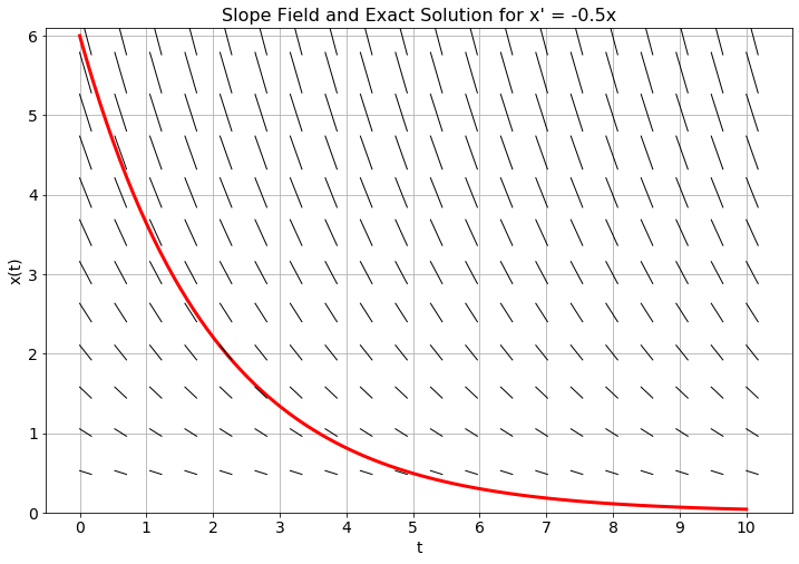
Figure 5.1: Plot your approximate solution on top of the slope field and the exact solution.

Exercise 5.10 In Figure 5.2 you see the analytic solution at $x(0)=5$ and a slope field for an unknown differential equation.

Use the slope field and a step size of $\Delta t=1$ to plot approximate solution values at $t=1$, $t=2$, $\ldots$, $t=10$. Connect your points with straight lines. The collection of line segments that you just drew is an aproximation to the solution of the unknown differential equation.
Use the slope field and a step size of $\Delta t = 0.5$ to plot approximate solution avlues at $t=0.5$, $t=1$, $t=1.5$, $\ldots$, $t=10$. Again, connect your points with straight lines to get an approximation of the solution to the unknown differential equation.
If you could take $\Delta t$ to be very very small, what difference would you see graphically between the exact solution and your collection of line segments? Why?

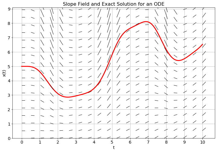
Figure 5.2: Plot your approximate solution on top of the slope field and the exact solution.

The notion of approximating solutions to differential equations is simple in principle:

make a discrete approximation to the derivative and
step forward through time as a difference equation.

The challenging part is making the approximation to the derivative(s). There are many methods for approximating derivatives, and that is exactly where we’ll start.

Definition 5.4 (Euler’s Method)Euler’s Method is a technique for approximating the solution to the differential equation $x'(t) = f(t,x(t))$. Recall from Problem 3.11 that the first derivative of a function can be discretized as \[x'(t) = \frac{x(t+h) - x(t)}{h} + \mathcal{O}(h)\] where $h = \Delta t$ is the step size (or the size of each partition in the domain), so the differential equation $x'(t) = f(t,x(t))$ becomes \[\frac{x(t+h) - x(t)}{h} \approx f(t,x(t)).\] Rewriting as a difference equation, letting $x_{n+1} = x(t_n+h)$ and $x_n = x(t_n)$, we get \[\begin{aligned} x_{n+1} = x_n + h f(t_n,x_n) \label{eqn:Eulers_method} \end{aligned}\]

A way to think about Euler’s method is that at a given point, the slope is approximated by the value of the right-hand side of the differential equation and then we step forward $h$ units in time following that slope. Figure 5.3 shows a depiction of the idea. Notice in the figure that in regions of high curvature Euler’s method will overshoot the exact solution to the differential equation. However, taking the limit as $h$ tends to $0$ theoretically gives the exact solution at the trade off of needing infinite computational resources.

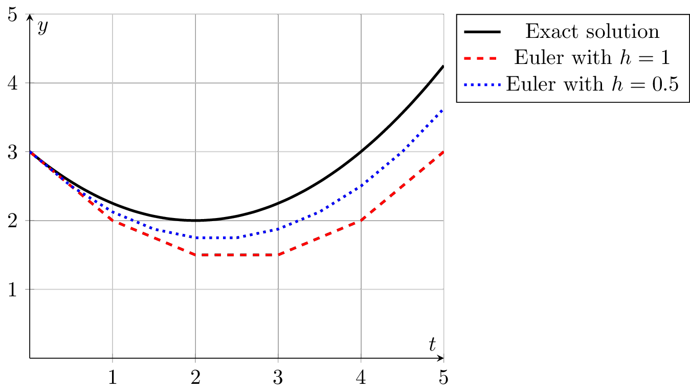
Figure 5.3: Numerical solutions to a differential equation using Euler’s method.

Exercise 5.11 Why would Euler’s method overshoot the exact solution in regions where the solution exhibits high curvature?

Exercise 5.12 Write code to implement Euler’s method for initial value problems. Your function should accept as input a Python function $f(t,x)$, an initial condition, a start time, an end time, and the value of $h = \Delta t$. The output should be vectors for $t$ and $x$ that you can easily plot to show the numerical solution. The code below will get you started.

def euler1d(f,x0,t0,tmax,dt):
    t = # set up the domain based on t0, tmax, and dt
    # next set up an array for x that is the same size a t
    x = np.zeros_like(t)
    x[0] = # fill in the initial condition
    for n in range( ??? ): # think about how far we should loop
        x[n+1] = # advance the solution forward in time with Euler
    return t, x

Exercise 5.13 Test your code from the previous exercise on a first order differential equation where you know the answer. Then test your code on the differential equation \[x' = -\frac{1}{3}x+\sin(t) \quad \text{where} \quad x(0) = 1.\] The partial code below should get you started.

import numpy as np
import matplotlib.pyplot as plt
# put the f(t,x) function on the next line 
# (be sure to specify t even if it doesn't show up in your ODE)
f = lambda t, x: # your function goes here
x0 = # initial condition
t0 = # initial time
tmax = # final time (your choice)
dt = # Delta t (your choice, but make it small)
t, x = euler1d(f,x0,t0,tmax,dt)
plt.plot(t,x,'b-')
plt.grid()
plt.show()

Exercise 5.14 The differential equation $x' = -\frac{1}{3}x + \sin(t)$ with $x(0) = 1$ has an analytic solution \[x(t) = \frac{1}{10} \left( 19 e^{-t/3} + 3\sin(t) - 9\cos(t) \right).\] The goal of this problem will be to compare the maximum error on the interval $t \in [0,5]$ for various values of $\Delta t$ in your Euler solver.

Write code that gives the maximum point-wise error between your numerical solution and the analytic solution given a value of $\Delta t$.
Using your code from part (a), build a plot with the value of $\Delta t$ on the horizontal axis and the value of the associated error on the vertical axis. You should use a log-log plot. Obviously you will need to run your code many times at many different values of $\Delta t$ to build your data set.
In general, if you were to cut your value of $\Delta t$ in half, what would that do to the value of the error? What about dividing $\Delta t$ by 10? 100? 1000?

Exercise 5.15 Shelby solved a first order ODE $x' = f(t,x)$ using Euler’s method with a step size of $dt = 0.1$ on a domain $t \in [0,3]$. To test her code she used a differential equation where she new the exact analytic solution and she found the maximum absolute error on the interval to be $0.15$. Jackson then solves the exact same differential equation, on the same interval, with the same initial condition using Euler’s method and a step size of $dt = 0.01$. What is Jackson’s expected maximum absolute error?

Theorem 5.2 Euler’s method is a first order method for approximating the solution to the differential equation $x' = f(t,x)$. Hence, if the step size $h$ of the partition of the domain were to be divided by some positive constant $M$ then the maximum absolute error between the numerical solution and the exact solution would ???
(Complete the last sentence.)

Exercise 5.16 If we want to numerically solve the first order differential equation $x' = f(t,x)$ on the interval $t \in [0,1]$ with Euler’s method so that we realize a maximum absolute error of $10^{-8}$ between the numerical solution and the exact solution, then how many points do we need to subdivide the interval $[0,1]$ into?

Exercise 5.17 If a mass is hanging from a spring then Newton’s second law, $\sum F=ma$, gives us the differential equation $mx'' = F_{restoring} + F_{damping}$ where $x$ is the displacement of the mass from equilibrium, $m$ is the mass of the object hanging from the spring, $F_{restoring}$ is the force pulling the mass back to equilibrium, and $F_{damping}$ is the force due to friction or air resistance that slows the mass down.

Which of the following is a good candidate for a restoring force in a spring? Defend your answer.
1. $F_{restoring} = kx$: The restoring force is proportional to the displacement away from equilibrium.
2. $F_{restoring} = kx'$: The restoring force is proportional to the velocity of the mass.
3. $F_{restoring} = kx''$: The restoring force is proportional to the acceleration of the mass.
Which of the following is a good candidate for a damping force in a spring? Defend your answer.
1. $F_{damping} = bx$: The damping force is proportional to the displacement away from equilibrium.
2. $F_{damping} = bx'$: The damping force is proportional to the velocity of the mass.
3. $F_{damping} = bx''$: The damping force is proportional to the acceleration of the mass.
Put your answers to parts (a) and (b) together and simplify to form a second-order differential equation for position: \[ \underline{\hspace{0.25in}} x'' + \underline{\hspace{0.25in}} x' + \underline{\hspace{0.25in}} x = 0 \]
If we want to solve a second order differential equation numerically we need to convert it to first order differential equations (Euler’s method is only designed to deal with first order differential equations, not second order). To do so we can introduce a new variable, $x_1$, such that $x_1 = x'$. For the sake of notational consistency we define $x_0 = x$. The result is a system of first-order differential equations. \[\begin{aligned} x_0' &= x_1 \\ x_1' &= \underline{\hspace{2in}} \end{aligned}\]
The code and Euler’s method algorithm that we’ve created thus far in this chapter are only designed to work with a single differential equation instead of a system, so we need to make some modifications. We can discretize the system of differential equations using Euler’s method so that \[ \boldsymbol{x}' = F(t,\boldsymbol{x}) \] where $F$ is a function that accepts a vector of inputs, plus time, and returns a vector of outputs. In the context of this particular problem, \[ F(t,\boldsymbol{x}) = \begin{pmatrix} x_0' \\ x_1' \end{pmatrix} = \begin{pmatrix} x_1 \\ \underline{\hspace{1in}} \end{pmatrix} \]
We now need to discretize the derivatives in the system. As with 1D Euler’s method, we will use a first-order approximation of the first derivative so that \[ \frac{\boldsymbol{x}_{n+1} - \boldsymbol{x}_n }{h} = F(t_n,\boldsymbol{x}_n) + \mathcal{O}(h). \] Rearranging and solving for $\boldsymbol{x}_{n+1}$ gives \[ \boldsymbol{x}_{n+1} = \underline{\hspace{0.5in}} + h F( \underline{\hspace{0.25in}} , \underline{\hspace{0.25in}}). \]
We now have a choice about how we’re going to code this new 2D version of Euler’s method. We could just include one more input function and one more input initial condition into the euler() function so that the Python function call is euler(f0,f1,x0,x1,t0,tmax,dt) where f0 and f1 are the two right-hand sides of the system, and x0 and x1 are the two initial conditions. Alternatively, we could rethink our euler() function so that it accepts an array of functions and an array of initial conditions so that the Python function call is euler(F,X,t0,tmax,dt) where F is a Python array of functions and X is a Python array of initial conditions. Discuss the pros and cons of each approach.
The following Python function and associated script will implement the vector version of Euler’s method. Complete the code and then use it to solve the system of equations from part (d). Use a mass of $m=2$kg, a damping force of $b=40$kg/s, and a spring constant of $k=128$N/m. Consider an initial position of $x=0$m (equilibrium) and an initial velocity of $x_1 = 0.6$m/s. Show two plots: a plot that shows both position and velocity vs time and a second plot, called a phase plot, that shows position vs velocity.

def euler(F,x0,t0,tmax,dt):
    t = # same code as before to set up a vector for time
    # Next we set up x so that it is an array where the columns 
    # are the different dimensions of the problem.  For example, 
    # in this problem there will be 2 columns and len(t) rows
    x = np.zeros( (len(t), len(x0)) ) 
    x[0,:] = x0 # store the initial condition in the first row
    for n in range(len(t)-1):
        x[n+1,:] = x[ ??? , ??? ] + dt*F(t[ ??? ], x[ ??? , ??? ])
    return t, x

To use the euler() function defined above we can use the following code. Fill in the code for this system of differential equations with this problem.

F = lambda t, x: np.array([ x[1] , ??? ])
x0 = [ ??? , ??? ] # initial conditions
t0 = 0
tmax = 5 # pick something reasonable here
dt = 0.01 # your choice.  pick something small
t, x = euler(F,x0,t0,tmax,dt)
# Next we plot the solutions against time 
plt.plot(t,x[ ??? , ???],'b-',t,x[ ??? , ???],'r--')
plt.grid()
plt.title('Time Evolution of Position and Velocity')
plt.legend(['which legend entry here','which legend entry here'])
plt.xlabel('time')
plt.ylabel('position and velocity')
plt.show()
# Then we plot one solution against the other for a phase plot
# In a phase plot time is implicit (not one of the axes)
plt.plot(x[ ??? , ???], x[ ??? , ???], 'k--')
plt.grid()
plt.title('Phase Plot')
plt.xlabel('???')
plt.ylabel('???')
plt.show()

Exercise 5.18 Consider a collection of two connected mass-spring oscillators where there is a mass hanging from a fixture and a second mass is connected directly to the first (hanging vertically). For simplicity in this problem we will neglect damping. Let $k_0$ and $k_1$ be the spring constants for the two springs, respectively. Also let $m_0$ and $m_1$ be the respective masses. For simplicity in this problem we will take $m_0 = m_1 = m$.

Draw a picture of the physical setup described. Let $x_0$ be the position of mass 0 relative to its equilibrium. Let $x_1$ be the position of mass 1 relative to its equilibrium. Label the coordinate systems for the two springs on your picture.
Give a thorough explanation for why the following second order differential equation models the position of the first mass \[ m x_0'' = -k_0 x_0 - k_1 (x_0 - x_1). \]
Using similar logic from part (b), write a second order differential equation for the position of the second mass \[ m x_1'' = \underline{\hspace{2in}} \]
We now have a system of two second order differential equations. We can convert this to four first order differential equations by introducing two new variables: $x_2 = x_0'$ and $x_3 = x_1'$. Write the full system of first order differential equations.
Use your vector-based euler() function to numerically solve the system of equations in several different physical scenarios. There are four variables so you will need to think carefully about which plots are the most explanatory. Also, if may be easiest to take $k_0 = 1$ and then take $k_1$ as the stiffness of spring 1 relative to spring 0 (e.g. if $k_1 = 1$ then the springs are the same stiffness, if $k_1 = 0.5$ then spring 1 is half as stiff, etc). To start with choose $m=m_0 = m_1 = 1$kg.

Exercise 5.19 Extend the previous exercise to that there are three masses hanging in a chain.

Exercise 5.20 If the speed of the mass in the mass-spring oscillator is fast enough then the damping force will no longer just be proportional to the velocity. Instead, at higher speeds the drag force is proportional to the square of the velocity. You can think of this as a bungee jumper jumping off of a bridge. Modify the single mass-spring oscillator equation to allow for nonlinear quadratic damping. Solve the system numerically under several different physical conditions (stiff spring, non-stiff spring, high damping, low damping, different initial conditions, etc).

Exercise 5.21 (A Lotka-Volterra Model) Test your code from the previous problems on the following system of differential equations by showing a time evolution plot (time on $x_0$ and populations on $x_1$) as well as a phase plot ($x_0$ on the $x$ and $x_1$ on the $y$ with time understood implicitly):
The Lotka-Volterra Predator-Prey Model:
Let $x_0(t)$ denote the number of rabbits (prey) and $x_1(t)$ denote the number of foxes (predator) at time $t$. The relationship between the species can be modeled by the classic 1920’s Lotka-Volterra Model: \[\left\{ \begin{array}{ll} x_0' &= \alpha x_0 - \beta x_0 x_1 \\ x_1' &= \delta x_0 x_1 - \gamma x_1 \end{array} \right.\] where $\alpha, \beta, \gamma,$ and $\delta$ are positive constants. For this problems take $\alpha \approx 1.1$, $\beta \approx 0.4$, $\gamma \approx 0.1$, and $\delta \approx 0.4$.

First rewrite the system of ODEs in the form $\boldsymbol{x}' = F(t,\boldsymbol{x})$ so you can use your euler() code.
Modify your code from the previous problem so that it works for this problem. Use tmax = 200 and an appropriately small time step. Start with initial conditions $x_0(0)=20$ rabbits and $x_1(0)=1$ fox.
Create the time evolution plot. What does this plot tell you in context?
Create a phase plot. What does this plot tell you in context?
If you cut your time step in half, what do you see in the two plots? Why? What is Euler’s method doing here?

Exercise 5.22 (The SIR Model) A classic model for predicting the spread of a virus or a disease is the SIR Model. In these models, $S$ stands for the proportion of the population which is susceptible to the virus, $I$ is the proportion of the population that is currently infected with the virus, and $R$ is the proportion of the population that has recovered from the virus. The idea behind the model is that

Susceptible people become infected by hanving interaction with the infected people. Hence, the rate of change of the susceptible people is proportional to the number of interactions that can occur between the $S$ and the $I$ populations.
\[ S' = -\alpha SI \]
The infected population gains people from the interactions with the susceptible people, but at the same time, infected people recover at a predictable rate. \[ I' = \alpha SI - \beta I \]
The people in the recovered class are then immune to the virus, so the recovered class $R$ only gains people from the recoveries from the $I$ class. \[ R' = \beta I \]

Explain the minus sign in the $S'$ equation in the context of the spread of a virus.
Explain the product $SI$ in the $S'$ equation in the context of the spread of a virus.
Find a numerical solution to the system of equations using your euler() function. Use the parameters $\alpha = 0.4$ and $\beta = 0.04$ with initial conditions $S(0) = 0.99$, $I(0) = 0.01$, and $R(0) = 0$. Explain all three curves in context.

5.4 The Midpoint Method

Now we get to improve upon Euler’s method. There is a long history of wonderful improvements to the classic Euler’s method – some that work in special cases, some that resolve areas where the error is going to be high, and some that are great for general purpose numerical solutions to ODEs with relatively high accuracy. In this section we’ll make a simple modification to Euler’s method that has a surprisingly great payoff in the error rate.

Exercise 5.23 In Euler’s method, if we are at the point $t_n$ then we approximate the slope $x'(t_n) = f(t_n,x_n)$ and use the slope to propagate forward one time step. As you have seen, this method can lead to an overshooting of the exact solution in regions of high curvature. It would be nice to be able to look into the future and get a better approximation of the slope so that we didn’t miss upcoming curvature. If you could build such a method that looks in to the future, finds a slope in the future, and then uses that slope (instead of the slope from Euler’s method) to advance forward in time, how far into the future would you look? Why?

Exercise 5.24 Let’s return to the simple differential equation $x' = -0.5x$ with $x(0) = 6$ that we saw in Exercise 5.9. Now we’ll propose a slightly different method for approximating the solution.

At $t=0$ we know that $x(0)=6$. If we use the slope at time $t=0$ to step forward in time then we will get the Euler approximation of the solution. Consider this alternative approach:

Use the slope at time $t=0$ and move half a step forward.
Find the slope at the half-way point
Then use the slope from the half way point to go a full step forward from time $t=0$.

Perhaps a bit confusing …let’s build this idea together:

What is the slope at time $t=0$? $x'(0) = \underline{\hspace{0.5in}}$
Use this slope to step a half step forward and find the $x$ value: $x(0.5) \approx \underline{\hspace{0.5in}}$
Now use the differential equation to find the slope at time $t=0.5$. $x'(0.5) = \underline{\hspace{0.5in}}$
Now take your answer from the previous step, and go one full step forward from time $t=0$. What $x$ value do you end up with?
Your answers to the previous bullets should be: $x'(0) = -3$, $x(0.5) \approx 4.5$, $x'(0.5) = -2.25$, so if we take a full step forward with slope $m=-2.25$ starting from $t=0$ we get $x(1) \approx 3.75$.

Repeat the process outlined in part (a) to approximate the solution to the differential equation at times $t=2, 3, \ldots, 10$. Also record the exact answer at each of these times by noting that the exact solution is $x(t) = 6e^{-0.5t}$.

$t$	0	1	2	3	4	5	6	7	8	9	10
Euler approx of $x(t)$	6
New approx of $x(t)$	6
Exact value of $x(t)$	6

Draw a clear picture of what this method is doing in order to approximate the slope at each individual step.
How does your approximation compare to the Euler approximation that you found in Exercise 5.9?

Definition 5.5 (The Midpoint Method) The midpoint method is defined by first taking a half step with Euler’s method to approximate a solution at time $t_{n+1/2}$ There is not grid point at $t_{n+1/2}$ so we define this as $t_{n+1/2} = (t_n + t_{n+1})/2$. We then take a full step using the value of $f$ at $t_{n+1/2}$ and the approximate $x_{n+1/2}$. \[\begin{aligned} x_{n+1/2} &= x_n + \frac{h}{2} f(t_n,x_n) \\ x_{n+1} &= x_n + h f(t_{n+1/2},x_{n+1/2}) \end{aligned}\] Note: Indexing by $1/2$ in a computer is nonsense. Instead, we implement the midpoint method with: \[\begin{aligned} m_n &= f(t_n,x_n) \\ x_{temp} &= x_n + \frac{h}{2} m_n \\ x_{n+1} &= x_n + h f\left( t_n + \frac{\Delta t}{2}, x_{temp}\right) \end{aligned}\]

Exercise 5.25 Complete the code below to implement the midpoint method in one dimension.

def midpoint1d(f,x0,t0,tmax,dt):
    t = # build the times
    x = # build an array for the x values
    x[0] = # build the initial condition
    # On the next line: be careful about how far you're looping
    for n in range( ??? ): 
        # The interesting part of the code goes here.
    return t, x

Test your code on several differential equations where you know the solution (just to be sure that it is working).

f = lambda t, x: # your ODE right hand side goes here
x0 = # initial condition
t0 = 0
tmax = # ending time (up to you)
dt = # pick something small
t, x = midpoint1d( ??? , ??? , ??? , ??? , ??? )
plt.plot( ??? , ??? , ??? )
plt.grid()
plt.show()

Exercise 5.26 The goal in building the midpoint method was to hopefully capture some of the upcoming curvature in the solution before we overshot it. Consider the differential equation $x' = -\frac{1}{3}x + \sin(t)$ with initial condition $x(0) = 1$ on the domain $t \in [0,4]$. First get a numerical solution with Euler’s method using $\Delta t = 0.1$. Then get a numerical solution with the midpoint method using the same value for $\Delta t$. Plot the two solutions on top of each other along with the exact solution \[ x(t) = \frac{1}{10} \left( 19e^{-t/3} + 3\sin(t) - 9\cos(t) \right). \] What do you observe? What do you observe if you make $\Delta t$ a bit larger (like 0.2 or 0.3)? What do you observe if you make $\Delta t$ very very small (like 0.001 or 0.0001)?

There are several key takeaways from this problem. Discuss.

Exercise 5.27 Repeat Exercise 5.14 with the midpoint method. Compare your results to what you found with Euler’s method.

Exercise 5.28 We have studied two methods thus far: Euler’s method and the Midpoint method. In Figure 5.4 we see a graphical depiction of how each method works on the differential equation $y' = y$ with $\Delta t = 1$ and $y(0) = 1$. The exact solution at $t=1$ is $y(1) = e^1 \approx 2.718$ and is shown in red in each figure. The methods can be summarized in the table below.

Discuss what you observe as the pros and cons of each method based on the table and on the Figure.

Euler’s Method	Midpoint Method
1. Get the slope at time $t_n$	1. Get the slope at time $t_n$
2. Follow the slope for time $\Delta t$	2. Follow the slope for time $\Delta t/2$
	3. Get the slope at the point $t_n + \Delta t/2$
	4. Follow the new slope from time $t_n$ for time $\Delta t$

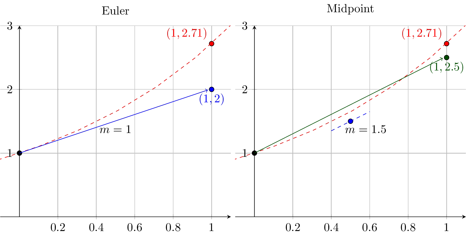
Figure 5.4: Graphical depictions of two numerical methods: Euler (left) and Midpoint (right). The exact solution is shown in red.

Exercise 5.29 When might you want to use Euler’s method instead of the midpoint method? When might you want to use the midpoint method instead of Euler’s method?

Exercise 5.30 (Midpoint Method in Several Dimensions) Modify your euler() code from Exercise 5.17 so that you can use the midpoint method in as many dimensions as you like. You should only have to add one line of code and then be careful about the size of the arrays that are in play. Test your code on several problems. Compare and contrast what you see with your Euler solutions and with your Midpoint solutions.

5.5 The Runge-Kutta 4 Method

OK. Ready for some experimentation? We are going to build a few experiments that eventually lead us to a very powerful method for finding numerical solutions to first order differential equations.

Exercise 5.31 Let’s talk about the Midpoint Method for a moment. The geometric idea of the midpoint method is outlined in the bullets below. Draw a picture along with the bullets.

You’re sitting at the point $(t_n,x_n)$.
The slope of the solution curve to the ODE where you’re standing is \[ \text{slope at the point $(t_n,x_n)$ is: } m_n = f(t_n,x_n) \]
You take a half a step forward using the slope where you’re standing. The new point, denoted $x_{n+1/2}$, is given by \[ \text{location a half step forward is: } x_{n+1/2} = x_n + \frac{\Delta t}{2} m_n. \]
Now you’re standing at $(t_n + \frac{\Delta t}{2} , x_{n+1/2})$ so there is a new slope here given by \[ \text{slope after a half of an Euler step is: } m_{n+1/2} = f(t_n+\Delta t/2,x_{n+1/2}). \]
Go back to the point $(t_n,x_n)$ and step a full step forward using slope $m_{n+1/2}$. Hence the new approximation is \[ x_{n+1} = x_n + \Delta t \cdot m_{n+1/2} \]

Exercise 5.32 One of the troubles with the midpoint method is that it doesn’t actually use the information at the point $(t_n,x_n)$. Moreover, it doesn’t leverage a slope at the next time step $t_{n+1}$. Let’s see what happens when we try a solution technique that combined the ideas of Euler and Midpoint as follows:

The slope at the point $(t_n,x_n)$ can be called $m_n$ and we find it by evaluating $f(t_n,x_n)$.
The slope at the point $(t_{n+1/2}, x_{n+1/2})$ can be called $m_{n+1/2}$ and we find it by evaluating $f(t_{n+1/2}, x_{n+1/2})$.
We can now take a full step using slope $m_{n+1/2}$ to get the point $x_{n+1}$ and the slope there is $m_{n+1} = f(t_{n+1}, x_{n+1})$.
Now we have three estimates of the slope that we can use to actually propagate forward from $(t_n,x_n)$:
- We could just use $m_n$. This is Euler’s method.
- We could just use $m_{n+1/2}$. This is the midpoint method.
- We could use $m_{n+1}$. Would this approach be any good?
- We could use the average of the three slopes.
- We could use a weighted average of the three slopes where some preference is given to some slopes over the others.

In the code below you will find a function called ode_test() that you can use as a starting point to test our the last three ideas. After the function you will see several lines of code that test your method against the differential equation $x'(t) = -\frac{1}{3}x + \sin(t)$ with $x(0) = 1$. The plots that come out are our typical error plots with the step size on the horizontal axis and our maximum absolute error between the numerical solution and the exact solution on the vertical axis. Recall that the exact solution to this differential equation is \[ x(t) = \frac{1}{10} \left( 19 e^{-t/3} + 3\sin(t) - 9\cos(t) \right) \]

import numpy as np
import matplotlib.pyplot as plt

# *********
# You should copy your euler and midpoint functions here. 
# We will be comparing to these two existing methods.
# *********

def ode_test(f,x0,t0,tmax,dt):
    t = np.arange(t0,tmax+dt,dt) # set up the times
    x = np.zeros(len(t)) # set up the x
    x[0] = x0 # initial condition
    for n in range(len(t)-1):
        m_n = f(t[n],x[n])
        x_n_plus_half = x[n] + (dt/2)*m_n
        m_n_plus_half = f( t[n]+dt/2 , x_n_plus_half )
        x_n_plus_1 = x[n] + dt * m_n_plus_half
        m_n_plus_1 = f(t[n]+dt, x_n_plus_1 )
        estimate_of_slope = # This is where you get to play
        x[n+1] = x[n] + dt * estimate_of_slope
    return t, x


f = lambda t, x: -(1/3.0)*x + np.sin(t)
exact = lambda t: (1/10.0)*(19*np.exp(-t/3) + \
                  3*np.sin(t) - \
                  9*np.cos(t))

x0 = 1 # initial condition
t0 = 0 # initial time
tmax = 3 # max time
# set up blank arrays to keep track of the maximum absolute errorrs
err_euler = [] 
err_midpoint = []
err_ode_test = []
# Next give a list of Delta t values (what list did we give here)
H = 10.0**(-np.arange(1,7,1)) 
for dt in H:
    # Build an euler approximation
    t, xeuler = euler(f,x0,t0,tmax,dt) 
    # Measure the max abs error
    err_euler.append( np.max( np.abs( xeuler - exact(t) ) ) ) 
    # Build a midpoint approximation
    t, xmidpoint = midpoint(f,x0,t0,tmax,dt) 
    # Measure the max abs error
    err_midpoint.append( np.max( np.abs( xmidpoint - exact(t) ) ) ) 
    # Build your new approximation
    t, xtest = ode_test(f,x0,t0,tmax,dt) 
    # Measure the max abs error
    err_ode_test.append( np.max( np.abs( xtest - exact(t) ) ) ) 

# Finally, we make a loglog plot of the errors.  
# Keep an eye on the slopes since they tell you the order of 
# the error for the method.
plt.loglog(H,err_euler,'r*-',
           H,err_midpoint,'b*-',
           H,err_ode_test,'k*-')
plt.grid()
plt.legend(['euler','midpoint','test method'])
plt.show()

Exercise 5.33 In the previous exercise you should have found that an average of the three slopes did just a little bit better than the midpoint method but the order of the error (the slope in the loglog plot) stayed about the same. You should have also found that the weighted average \[ \text{estimate of slope} = \frac{m_n + 2m_{n+1/2} + m_{n+1}}{4} \] did just a little bit better than just a plain average. Why might this be? (If you haven’t tried this weighted average then go back and try it.) Do other weighted averages of this sort work better or worse? Does it appear that we can improve upon the order of the error (the slope in the loglog plot) using any of these methods?

Exercise 5.34 OK. Let’s make one more modification. What if we built a fourth slope that resulted from stepping a half step forward using $m_{n+1/2}$? We’ll call this $m_{n+1/2}^*$ since it is a new estimate of $m_{n+1/2}$. \[ x_{n+1/2}^* = x_n + \frac{\Delta t}{2} m_{n+1/2} \] \[ m_{n+1/2}^* = f(t_n + \Delta t/2, x_{n+1/2}^*) \] Then calculate $m_{n+1}$ using this new slope instead of what we did in the previous problem.

Draw a picture showing where this slope was calculated.
Modify the code from above to include this fourth slope.
Experiment with several ideas about how to best combine the four slopes: $m_n$, $m_{n+1/2}$, $m_{n+1/2}^*$, and $m_{n+1}$.
- Should we just take an average of the four slopes?
- Should we give one or more of the slopes preferential treatment and do some sort of weighted average?
- Should we do something else entirely?

Remember that we are looking to improve the slope in the loglog plot since that indicates an improvement in the order of the error (the accuracy) of the method.

Exercise 5.35 In the previous exercise you no doubt experimented with many different linear combinations of $m_n$, $m_{n+1/2}$, $m_{n+1/2}^*$, and $m_n$. Many of the resulting numerical ODE methods likely had the same order of accuracy (again, the order of the method is the slope in the error plot), but some may have been much better or much worse. Work with your team to fill in the following summary table of all of the methods that you devised. If you generated linear combinations that are not listed below then just add them to the list (we’ve only listed the most common ones here).

	$m_n$	$m_{n+1/2}$	$m_{n+1/2}^*$	$m_n$	Order of Error	Name
1	1	0	0	0	$\mathcal{O}(\Delta t)$	Euler’s Method
2	0	1	0	0	$\mathcal{O}(\Delta t^2)$	Midpoint Method
3	1/2	1/2	0	0
4	1/3	1/3	0	1/3
5	1/4	2/4	0	1/4
6	0	0	1	0
7	0	1/2	1/2	0
8	1/3	1/3	1/3	0
9	1/4	1/4	1/4	1/4
10	1/5	2/5	1/5	1/5
11	1/5	1/5	2/5	1/5
12	1/6	2/6	2/6	1/6
13	1/6	3/6	1/6	1/6
14	1/6	1/6	3/6	1/6
15	1/7	2/7	3/7	1/7
16	1/8	3/8	3/8	1/8
17
18

Exercise 5.36 In the previous exercise you should have found at least one of the many methods to be far superior to the others. State which linear combination of slopes seems to have done the trick, draw a picture of what this method does to numerically approximate the next slope for a numerical solution to an ODE, and clearly state what the order of the error means about this method.

Theorem 5.3 (The Runge-Kutta 4 Method) The Runge-Kutta 4 (RK4) method for approximating the solution to the differential equation $x' = f(t,x)$ approximates the slope at the point $t_n$ by using the following weighted sum: \[ \text{estimated slope } = \frac{m_n + 2 m_{n+1/2} + 2 m_{n+1/2}^* + m_n}{6}. \] The order of the error in the RK4 method is $\mathcal{O}(\Delta t^4)$.

Exercise 5.37 In Theorem 5.3 we state the Runge-Kutta 4 method in terms of the estimates of the slope built up previously in this section. The notation that is commonly used in most numerical analysis sources is slightly different. Typically, the RK4 method is presented as follows: \[\begin{aligned} k_1 &= f(t_n, x_n) \\ k_2 &= f(t_n + \frac{h}{2}, x_n + \frac{h}{2} k_1) \\ k_3 &= f(t_n + \frac{h}{2}, x_n + \frac{h}{2} k_2) \\ k_4 &= f(t_n + h, x_n + h k_3) \\ x_{n+1} &= x_n + \frac{h}{6} \left( k_1 + 2 k_2 + 2 k_3 + k_4 \right) \end{aligned}\]

Show that indeed we have derived the same exact algorithm.
What is the advantage to posing the RK4 method in this way?
How many evaluations of the function $f(t,x)$ do we need to make at every time step of the RK4 method? Compare this Euler’s method and the midpoint method. Why is this important?

Exercise 5.38 Jackson wants to solve the differential equation $x' = f(t,x)$ on the domain $t \in [0,1]$ so that the maximum absolute error is less than $10^{-8}$.

What value of $\Delta t$ would Jackson need if he were using Euler’s method? How many function evaluations would Jackson’s Euler algorithm end up doing in order to achieve his desired level of accuracy.
What value of $\Delta t$ would Jackson need if he were using the midpoint method? How many function evaluations would Jackson’s midpoint algorithm end up doing in order to achieve his desired level of accuracy.
What value of $\Delta t$ would Jackson need if he were using the RK4 method? How many function evaluations would Jackson’s RK4 algorithm end up doing in order to achieve his desired level of accuracy.
Discuss the implications of what you found in parts (a) - (c) of this problem.

Exercise 5.39 It would nice, but it would be completely impractical, to have a numerical method compute the approximate solution so that the maximum absolute error is less than machine precision $10^{-16}$. That is an impracticality since we can’t actually detect errors that small on a computer using double precision arithmetic. However, what if we wanted accuracy of $10^{-15}$ instead? Repeat the previous exercise with $10^{-15}$ as the goal for the maximum absolute error.

Exercise 5.40 Let’s step back for a second and just see what the RK4 method does from a nuts-and-bolts point of view. Consider the differential equation $x' = x$ with initial condition $x(0) = 1$. The solution to this differential equation is clearly $x(t) = e^t$. For the same of simplicity, take $\Delta t = 1$ and perform 1 step of the RK4 method BY HAND to approximate the value $x(1)$.

Exercise 5.41 Write a Python function that implements the Runge-Kutta 4 method in one dimension. Test the problem on several differential equations where you know the solution.

import numpy as np
import matplotlib.pyplot as plt

def rk41d(f,x0,t0,tmax,dt):
    t = np.arange(t0,tmax+dt,dt)
    x = np.zeros_like(t)
    x[0] = x0
    for n in range(len(t)-1):
        # the interesting bits of the code go here
    return t, x

f = lambda t, x: -(1/3.0)*x + np.sin(t)
x0 = # initial condition
t0 = 0
tmax = # your choice
dt = # pick something reasonable
t, x = rk41d(f,x0,t0,tmax,dt)
plt.plot(t,x,'b.-')
plt.grid()
plt.show()

(**RK4 in Several Dimensions**) Modify your Runge-Kutta 4 code to work for any number of dimensions.  You may want to start from your `euler()` and `midpoint()` functions that already do this.  You'll only need to make minor modifications from there.  Then test your new generalized RK4 method on all of the same problems which you used to test your `euler()` and `midpoint()` functions.

5.6 Animating ODE Solutions

Differential equations that depend on time are often best visualized when they are animated. This can also be said about any parameterized function, but in this present case we will focus on visualizing differential equations. There are several animation tools with python and we’ll demonstrate only two primary technique here:

ipywidgets.interactive is a tool that will produce an image with sliders that can be used to manually control an animation. The big advantage to ipywidgets.iteractive is that you can animate over several parameters, and hence use this tool as a playground for learning how parameters interact with each other.
matplotlib.animation is a tool built directly into matplotlib that gives a playable animation (like a small movie). In this sort of animation we can only animate over one parameter or variable (like time), but this is most like what we would expect when animating a function that changes over time.

The reader should take careful note that the tools described here are meant to be used in Google Colab. These tools may not work as expected in other instances of Python and you may have to do some playing around (and Googling) to get it to work properly on your Python installation. Moreover, the animations are not built directly into the book since this book is delivered in several formats (HTML, PDF, and print). Instead you will find links to Google Colab documents that have the contain the code and animations.

5.6.1 `ipywidgets.interactive`

Consider the differential equation $x' = f(t,x)$ with $x(0) = x_0$. We would like to build an animation of the numerical solution to this differential equation over the parameters $t$ but also over $x_0$ and $\Delta t$. The following blocks of python code walk through this animation.

Example 5.2 (ipywidgets.interactive) Let’s say that we want to control the numerical solution to the differential equation $x' = -\frac{1}{3}x + \sin(t)$ by manually altering the values of $x(0) = x_0$, $t_{max}$, and $\Delta t$. In this case we will solve the differential equation using Euler’s method but note that our code could be easily modified to use other solvers.

First we import all of the appropriate libraries. Of particular interest is the ipywidgets.interactive library. This allows for images to be interactive with the use of sliders. Moving the sliders will provide a nice way to animate a plot manually.

from ipywidgets import interactive
import matplotlib.pyplot as plt
import numpy as np

In the next block of code we define our euler() solver. This particular step is only included because we are using Euler’s method to solve this specific problem. In general, include an functions or code that are going to be used to produce the data that you will be plotting. We will also introduce the function f and the parameter t0 since we will not be animating over these parameters.

def euler(f,x0,t0,tmax,dt):
  N = int(np.floor((tmax-t0)/dt)+1)
  t = np.linspace(t0,tmax,N+1)
  x = np.zeros_like(t)
  x[0] = x0
  for n in range(len(t)-1):
    x[n+1] = x[n] + dt*f(t[n],x[n])
  return t, x

f = lambda t, x: -(1/3.0)*x + np.sin(t)
t0 = 0

Next we build a function that accepts only the parameters that we want to animate over and produces only a plot. This function will be called later by the ipywidgets.interactive function every time we change one of the parameters so be sure that this is a clean and fast function to evaluate (keep the code simple).

def eulerAnimator(x0,tmax,dt):
    # call on the euler function to build the solution
    t, x = euler(f,x0,t0,tmax,dt) 
    plt.plot(t, x, 'b-') # plot the solution
    plt.xlim(0,30)
    plt.ylim( np.min(x)-1, np.max(x)+1)
    plt.grid()
    plt.show()

Now that we have everything set up we need to call on the ipywidgets.interactive command to turn the graphic into a visualization which can be controlled by sliders. In the code below we are allowing the initial condition to range between $x_0 = -2$ and $x_0 = 5$ in steps of $0.5$, the time to range from $t_{max}=1$ to $t_{max}=30$ in steps of $0.1$, and the time step to range from $\Delta t = 0.01$ to $\Delta t = 0.75$ in steps of $0.005$.

interactive_plot = interactive(eulerAnimator, 
                               x0=(-2, 5, 0.5), 
                               tmax=(1, 30, 0.1), 
                               dt=(0.01, 0.75, 0.005))
interactive_plot

A static snapshot of the animation applet is shown in Figure 5.5. When you build this animation you will have control over all three parameters. Like we mentioned before, this sort of animation can be a great playground for building insight into the interplay between parameters.

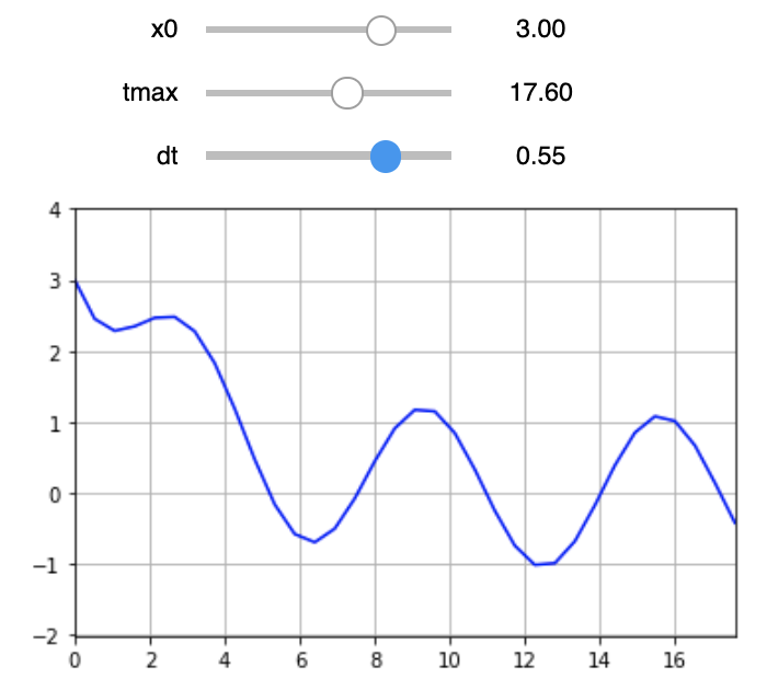
Figure 5.5: Snapshot of the ODE animation applet with ipywidgets.

Exercise 5.42 Modify the previous exercise to use a different numerical solver (e.g. the midpoint method) instead of Euler’s method.

Exercise 5.43 Modify the animation routine above to simultaneously show the Euler, Midpoint, and RK4 solutions to a differential equation on top of each other. Animate over different values of $\Delta t$ for fixed values of $x_0$ and $t_{max}$.

5.6.2 `matplotlib.animation`

The next animation package that we discuss is the matplotlib.animation package. This particular package is very similar to ipywidgets.interactive, but results only in a playable movie that is embedded within the Google Colab environment.

Exercise 5.44 Again we will consider the differential equation $x' = -\frac{1}{3}x + \sin(t)$ but this time we will only be interested in an animation over time.

We start the code by importing all of the necessary libraries. Take note that we import the matplotlib.animation and matplotlib.rc libraries in order to build the animation. We then import the IPython.display.HTML library to take care of embedding the player into the Google Colab environment.

import numpy as np
import matplotlib.pyplot as plt
from matplotlib import animation, rc
from IPython.display import HTML

Next we write all of the code necessary to build an Euler solution for the differential equation. Take note, of course, that much of this code is specific only to this problem and what we really need here is code that produces data for the animation.

def euler(f,x0,t0,tmax,dt): # this is the Euler function
  N = int(np.floor((tmax-t0)/dt)+1)
  t = np.linspace(t0,tmax,N+1)
  x = np.zeros_like(t)
  x[0] = x0
  for n in range(len(t)-1):
    x[n+1] = x[n] + dt*f(t[n],x[n])
  return t, x

# Now we define the parameters for the Euler function
dt = 1e-2
x0 = 3 # initial condition
t0 = 0
tmax = 10
f = lambda t, x: -(1/3.0)*x + np.sin(t)

# Next we get the full Euler solution associate with these 
# parameters.  Be careful that you put this outside your 
# animation loop so that you don't build this over and over.
t, x = euler(f,x0,t0,tmax,dt)

Next we have to set up the figure that we are going to animate. This involves:

setting up the axes,
building any features onto the axes that we want (e.g. a grid, axis labels, axis limits, etc)
and then we build a variable that we call frame.
- The variable frame contains a blank plot with no data.
- Notice that we define the line and marker styles here.
- Also notice the comma in the definition of the frame variable. This is here since there are several Python objects inside ax.plot() and we only want to unpack the first one into frame.

fig, ax = plt.subplots()
plt.close()
# Below we set up many of the global parameters for the plot.
# Much of what we do here depends on what we are trying to animate.
ax.grid()
ax.set_xlabel('Time')
ax.set_ylabel('Approximate Solution')
ax.set_xlim(( t0, tmax)) 
ax.set_ylim((np.min(x)-0.5, np.max(x)+0.5)) 
frame, = ax.plot([], [], linewidth=2, linestyle='--') 
# notice we also set line and marker parameters here

Now we build a function that accepts only the animation frame number, N, and adds appropriate elements to the plot defined by frame.

def animator(N): # N is the animation frame number
  T = t[:N] # get t data up to the frame number
  X = x[:N] # get x data up to the frame number
  # display the current simulation time in the title
  ax.set_title('Time='+t[N]) 
  # put the data for the current frame into the varable "frame"
  frame.set_data(T,X) 
  return (frame,)

In the next block of code we define which frames we want to use in the animation and then we call upon the matplotlib.animation function to build the animation.

# The Euler solution takes many very small time steps.  
# To speed up the animation we view every 10th iteration.
PlotFrames = range(0,len(t),10) 
anim = animation.FuncAnimation(fig, # call on the figure
# next call the function that builds the animation frame
                               animator, 
# next tell which frames to pass to animator
                               frames=PlotFrames, 
# lastly give the delay between frames                         
                               interval=100 
                               )

Finally, we embed the animation into the Google Colab environment. Take note that if you are using a different Python IDE then you may need to experiment with how to show the resulting animation.

rc('animation', html='jshtml') # embed in the HTML for Google Colab
anim # show the animation

A static snapshot of the resulting animation can be seen in Figure 5.6. The controls for the animation should be familiar from other media players.

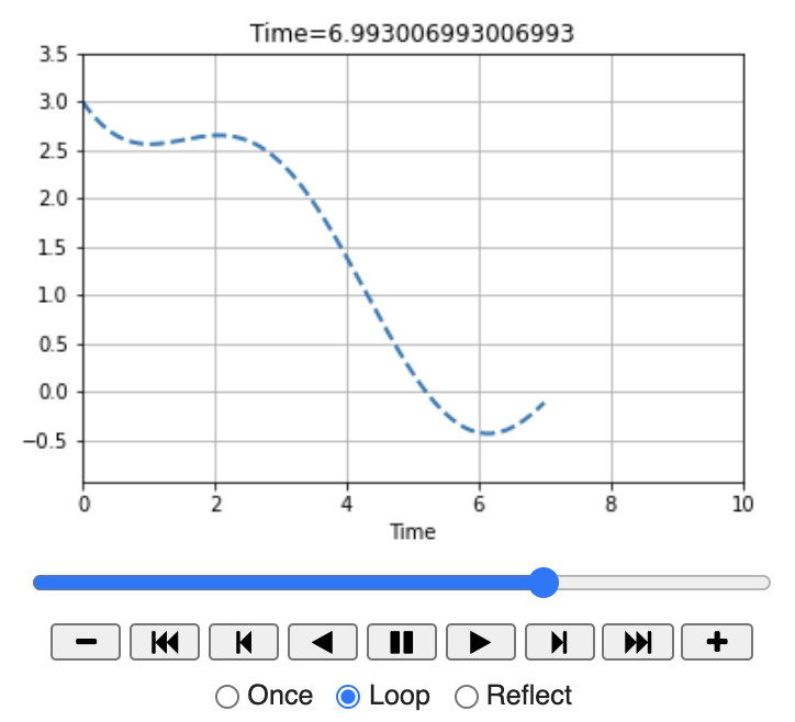
Figure 5.6: Snapshot of the ODE animation applet with matplotlib animation.

Exercise 5.45 Modify the code from the previous exercise to show faster and slower animations.

Exercise 5.46 Modify the matplotlib.animation code from Exercise 5.44 to use a different differential equation solver.

Exercise 5.47 Modify the matplotlib.animation code from Exericse 5.44 to show the Euler, Midpoint, and RK4 solutions to a differential equation on top of each other for a fixed value of $\Delta t$.

5.7 The Backwards Euler Method

We have now built up a fairly large variety of numerical ODE solvers. All of the solvers that we have built thus far are called explicit numerical differential equation solvers since they try to advance the solution explicitly forward in time. Wouldn’t it be nice if we could literally just say, what slope is going to work best in the future time steps … let’s use that? Seems like an unrealistic hope, but that is exactly what the last method covered in this section does.

Definition 5.6 (Backward Euler Method) We want to solve $x' = f(t,x)$ so:

Approximate the derivative by looking forward in time(!) \[\frac{x_{n+1} - x_n}{h} \approx f(t_{n+1}, x_{n+1})\]
Rearrange to get the difference equation \[x_{n+1} = x_n + h f(t_{n+1},x_{n+1}).\]
We will always know the value of $t_{n+1}$ and we will always know the value of $x_n$, but we don’t know the value of $x_{n+1}$. In fact, that is exactly what we want. The major trouble is that $x_{n+1}$ shows up on both sides of the equation. Can you think of a way to solve for it? …you have code that does this step!!!
This method is called the Backward Euler method and is known as an implicit method since you do not explicitly calculate $x_{n+1}$ but instead there is some intermediate calculation that needs to happen to solve for $x_{n+1}$. The (usual) advantage to an implicit method such as Backward Euler is that you can take far fewer steps with reasonably little loss of accuracy. We’ll see that in the coming problems.

Exercise 5.48 Let’s take a few steps through the backward Euler method on a problem that we know well: $x' = -0.5x$ with $x(0) = 6$.
Let’s take $h=1$ for simplicity, so the backward Euler iteration scheme for this particular differential equation is \[x_{n+1} = x_n - \frac{1}{2} x_{n+1}.\] Notice that $x_{n+1}$ shows up on both sides of the equation. A little bit of rearranging gives \[\frac{3}{2} x_{n+1} = x_n \quad \implies \quad x_{n+1} = \frac{2}{3} x_n.\]

Complete the following table.

$t$	0	1	2	3
Euler Approx. of $x$	6	3	1.5	0.75
Back. Euler Approx.of $x$	6	4	2.667	1.778
Exact value of $x$	6	3.64	2.207	1.339

Compare now to what we found for the midpoint method on this problem as well.

Exercise 5.49 The previous problem could potentially lead you to believe that the backward Euler method will always result in some other nice difference equation after some algebraic rearranging. That isn’t true! Let’s consider a slightly more complicated differential equation and see what happens \[x' = -\frac{1}{2} x^2 \quad \text{with} \quad x(0) = 0.\]

Recall that the backward Euler approximation is \[x_{n+1} = x_n + h f(t_{n+1},x_{n+1}).\] Let’s take $h=1$ for simplicity (we’ll make it smaller later). What is the backward Euler formula for this particular differential equation?
You should notice that your backward Euler formula is now a quadratic function in $x_{n+1}$. That is to say, if you are given a value of $x_n$ then you need to solve a quadratic polynomial equation to get $x_{n+1}$. Let’s be more explicit:
We know that $x(0) = 6$ so in our numerical solutions, $x_1 = 6$. In order to get $x_2$ we consider the equation $x_2 = x_1 - \frac{1}{2} x_2^2$. Rearranging we see that we need to solve $\frac{1}{2}x_2^2 + x_2 - 6 = 0$ in order to get $x_2$. Doing so gives us $x_2 = \sqrt{13} - 1 \approx 2.606$.
Go two steps further with the backward Euler method on this problem. Then take the same number of steps with regular (forward) Euler’s method.
Work our the analytic solution for this differential equation (using separation of variables perhaps). Then compare the values that you found in parts (b) and (c) of this problem to values of the analytic solution and values that you would find form the regular (forward) Euler approximation. What do you notice?

The complications with the backward Euler’s method are that you have a nonlinear equation to solve at every time step \[x_{n+1} = x_n + h f(t_{n+1},x_{n+1}).\] Notice that this is the same as solving the equation \[x_{n+1} - hf(t_{n+1},x_{n+1}) - x_n = 0.\] You know the values of $h=\Delta t$, $t_{n+1}$ and $x_n$, and you know the function $f$, so, in a practical sense, you should use some sort of Newton’s method iteration to solve that equation – at each time step. More simply, we could call upon scipy.optimize.fsolve() to quickly implement a built in Python numerical root finding technique for us.

Exercise 5.50 Consider the function backwardEuler1d() below. How do you define the function G inside the for loop and what seed do you use to start the fsolve() command?

import numpy as np
from scipy import optimize
def backwardEuler1d(f,x0,t0,tmax,dt):
    t = np.arange(t0,tmax+dt,dt)
    x = np.zeros_like(t)
    x[0] = x0
    for n in range(len(t)-1):
        G = lambda X: ??? # define this function
        # give the correct seed for the solver below
        x[n+1] = optimize.fsolve(G, ??? )[0] 
    return t, x

Exercise 5.51 Test the Backward Euler method from the previous problem on several differential equations where you know the solution.

Exercise 5.52 Write a script that outputs a log-log plot with the step size on the horizontal axis and the error in the numerical method on the vertical axis. Plot the errors for Euler, Midpoint, Runge Kutta, and Backward Euler measured against a differential equation with a known analytic solution. Use this plot to conjecture the convergence rates of the four methods. You can use the differential equation $x' = -\frac{1}{3} x + \sin(t)$ with $x(0) = 1$ like we have for many of our past algorithm since we know that the solution is \[ x(t) = \frac{1}{10}\left( 19e^{-t/3} + 3\sin(t) - 9\cos(t) \right) \]

Exercise 5.53 What is the order of the error on the Backward Euler method? Given this answer, what are the pros and cons of the Backward Euler method over the regular Euler method? What about compared to the Midpoint or Runge Kutta methods?

Exercise 5.54 It may not be obvious at the outset, but the Backward Euler method will actually behave better than our regular Euler’s method in some sense. Let’s take a look. Consider, for example, the really simply differential equation $x' = -x$ with $x(0) = 1$ on the interval $t \in [0,2]$. The analytic solution is $x(t) = e^{-t}$. Write Python code that plots the analytic solution, the Euler approximation, and the Backward Euler approximation on top of each other. Use a time step that is larger than you normally would (such as $\Delta t = 0.25$ or $\Delta t = 0.5$ or larger). Try the same experiment on another differential equation where we know the exact solution and the solution has some regions of high curvature. What do you notice? What does Backward Euler do that is an improvement on regular Euler?

5.8 Fitting ODE Models to Data

To end this chapter we will examine a very common scientific situation: We have data from an experiment and a (challenging to solve) differential equation modeling the data that has some parameter that controls the behavior. We want to find the value of the parameter that gives us the best fit between our numerical solution and the data. For example, say we have temperature data for a cooling liquid and we have a differential equation for temperature that depends on a parameter related to the thermal properties of the container. We would like to use the data and the differential equation to determine the parameter for the container. As another example, say we have the number of patients that become ill with a virus each day and we actually want to know the long-term impacts on the population. An SIR differential equation model might describe the dynamics of the situation well, and the data can be used to determine the transmission rate parameters in the model.

Data fitting has been examined a few times in this book (see the Least Squares section in Chapter 3 and the Over determined Systems section in Chapter 4). The present situation is really not that much different than regular least squares curve fitting.

Propose a model function: In this case our model function will be a numerical solution to a differential equation given some value for an unknown parameter.
Calculate the sum of the squared residuals: In this case, we need to match the times between the numerical solution and the data. There will likely be far more points in the numerical solution than there will be in the data so we will have to carefully select the points that closely match between the two. Then calculating the sum of the squared error is simple.
Use an optimization routine to find the value of the best parameter: In this case this is no different than regular least squares. We are trying to find the value of the parameter that minimizes the sum of the squared residuals.

Exercise 5.55 (Newton’s Law of Cooling) From Calculus you may recall Newton’s Law of Cooling: \[ \frac{dT}{dt} = -k(T - T_{ambient}) \] where $T$ is the temperature of some object (like a cup of coffee), $T_{ambient}$ is the temperature of the ambient environment, and $k$ is the proportionality constant that governs the rate of cooling. This is a classic differential equation with a well known solution.¹² In the present situation we don’t want the analytic solution, but instead we will work with a numerical solution since we are thinking ahead to where the differential equation may be very hard to solve in future problems. We also don’t want to just look at the data and guess an algebraic form for the function that best fits the data. That would be a trap! (why?) Instead, we rely on our knowledge of the physics of the situation to give us the differential equation.

The following data table gives the temperature (degrees $F$) at several times while a cup of tea cools on a table [7]. The ambient temperature of the room is $65^\circ F$.

Time (sec)	Temperature
0	160
60	155
180	145
210	142
600	120

Plot the data as a scatter plot.

import numpy as np
import pandas as pd
import matplotlib.pyplot as plt
URL1 = 'https://raw.githubusercontent.com/NumericalMethodsSullivan'
URL2 = '/NumericalMethodsSullivan.github.io/master/data/'
URL = URL1+URL2
data = np.array( pd.read_csv(URL+'Exercise5_newtoncooling.csv') )
# Exercise5_newtoncooling.csv
# 
# or you can load the data directly with 
# data = np.array([[0,160],[60,155],[180,145],[210,142],[600,120]])
plt.plot(data[??? , ???] , data[??? , ???], 'b*')
plt.grid()
plt.show()

Now we will build several Python functions as well as several additional lines of code that are created specifically for this problem. Note that every parameter estimate problem of this type will take similar form, but there may be subtle differences depending on the data that you need to account for in each problem. You will need to taylor make parts of each parameter estimation script for each new problem.

First we set the stage by defining $\Delta t$, a collection of times that contains the data, the function $f(t,x; k)$ which depends on the parameter $k$, and any other necessary parameters of our specific problem.

import numpy as np
Tambient = ???
# Next choose an appropriate value of dt.  
# Choosing dt so that values of time in the data fall within
# the times for the numerical solution is typically a good 
# practice (but is not always possible).
dt = ??? 
t0 = 0 # time where the data starts
tmax = ??? # just beyond where the data ends
t = np.arange(t0,tmax+dt,dt) # set up the times 
# nest we define our specific differential equation
f = lambda t, x, k: -k*(x - Tambient) 
x0 = ??? # initial condition pulled from the data

Now we build a Python function that will accept a value of the parameter $k$ as the only input and will return a high quality numerical solution to the proposed differential equation.

def numericalSolution(k):
    x = np.zeros_like(t)
    x[0] = x0
    for n in range(len(t)-1):
        # put the code necessary to build a good 
        # numerical solver here be sure to account 
        # for the parameter k in each of your function calls.
    return t, x

Spend a little time now playing with different parameters and plotting numerical solutions along with the data to determine the proper ballpark value of the parameter.
Now we need to write a short Python script that will find all of the indices where the value of time in the data closely match values of time in the numerical solution. There are many ways to do this, but the most readable is a pair of nested for loops. Outline what the following code does. Why are we using dt/2 in the code below? You should work to find more efficient ways to code this for bigger problems since the nested for loops is potentially quite time consuming.

indices = []
for j in range(len(t)):
    for k in range(len(data)):
        if # write a check to find where t is closest to data[:,1]
            indices.append(j)

Now we build a Python function dataMatcher(k) which accepts the parameter $k$ and outputs the sum of the squared residuals between the numerical solution associated with $k$ and our data. Carefully dissect the following code.

def dataMatcher(k):
    t, x = numericalSolution(k)
    err = []
    counter = 0
    for n in indices:
        err.append( (data[counter,1] - x[int(n)])**2 )
        counter += 1
    print("For k=",k[0],",  SSRes=",np.sum(err)) # optional
    return np.sum(err)

Test your dataMatcher() function to be sure that it is working properly on a value of $k$ which visually matches the data well.
Finally, we call upon the scipy.optimize.minimize() function to iteratively try different values of the parameter $k$ and to find the one that minimizes the sum of the squared residuals. Be sure to start $k$ at a value that gives a reasonably good visual match between the numerical solution and the data. Once the optimization routine is done you should plot your best solution on top of the data to verify that it indeed found a good solution. You’ll notice that there are several options that you can send to the scipy.optimize.minimize() command. Play with these options to see what they do and how they impact the quality of your solution.

import scipy.optimize as sp
# Choose an initial value of k and put it into the following code 
# in place of the "???".  Note that we are sending a few parameters 
# to the optimization tool.  Be sure to understand these options 
# and take care that these options problem dependent and you will 
# need to choose these again for the next new problem.
K = sp.minimize(dataMatcher,???, options = {'maxiter': 5}, tol=1e-2)
print(K)
t, x = numericalSolution(K.x[0])
plt.plot(t,x,'r--',data[:,0],data[:,1],'b*')
plt.grid()
plt.show()

Note: If your optimization does not terminate successfully then you’ll need to go back to the point where you guess a few values for the parameter so that your initial guess for scipy.optimize.minimize() is close to what it should be. It is always helpful to think about the physical context of the problem to help guide your understanding of which value(s) to choose for your parameter.

To recap:

We have data and a proposed differential equation with an unknown parameter.
We matched numerical solutions to the differential equation to the data for various values of the parameter.
We used an optimization routine to find the value of the parameter that minimized the sum of the squared residuals between the data and the numerical solution.

At this point you can now use the best numerical solution to answer questions about the scientific setup (e.g. extrapolation).

Exercise 5.56 In the paper Steeping Tea: A differential equations approach to a great cup of fruit tea [7], the authors give color data from photographs of tea that is steeping in a clear mason jar. The temperature data from the previous exercise in this section were taken from this paper.

Read the introduction, methods, and experimental setup in the paper.
Think carefully about the physics of the problem to propose a differential equation (NOT an algebraic function) which would best models the grayscale data found on page 3 of the paper. Your model will likely involve at least one unknown parameter.
Use the least squares data fitting routine outlined in the previous exercise to find the value(s) of your parameter(s) which will create a high quality match between the numerical solution to your ODE and the data.
Plot your solution curve along with the data.

Exercise 5.57 (Village Epidemic) (This exercise is modified from [8])

In the mid seventeenth century in a small village in England a form of the Plague spread from July 3 through October 20 in one year. We note three classes of individuals: Susceptible, Infective, and Removed. The latter group consists of those who have died from the disease or who developed an immunity from the disease, having already had the disease. We keep track of the following:

$S(t)=$ the number of Susceptibles on day $t$ of the epidemic. $S(0) = 235$.
$I(t)=$ the number of Infectives on day $t$ of the epidemic. $I(0)=14$
$R(t)=$ the number of Removeds on day $t$ of the epidemic. $R(0)=0$.

A standard $SIR$ model takes the form \[\begin{aligned} S' &= -\alpha SI \\ I' &= \alpha SI - \beta I \\ R' &= \beta I. \end{aligned}\]

Data was gathered on the outbreak and is shown in the table below.

Time (days)	Susceptibles	Infectives
0	235	14
16	201	22
31	153.5	29
47	121	21
62	108	8
78	97	8
109	83	0

Use the least squares fitting technique discussed in this section to find the parameters $\alpha$ and $\beta$ that minimize the sum of the squared residuals between a numerical solution of the $SIR$ model and the data. You can load the data directly with the code below.

Note: The total population is fixed.

import numpy as np
import pandas as pd
URL1 = 'https://raw.githubusercontent.com/NumericalMethodsSullivan'
URL2 = '/NumericalMethodsSullivan.github.io/master/data/'
URL = URL1+URL2
data = np.array( pd.read_csv(URL+'Exercise5_village.csv') )
# Exercise5_village.csv

Exercise 5.58 (Bedridden Boys Problem) (This problem is modified from [9])

A boarding school is a relatively closed community in which all students live on campus, teachers tend to live on or near campus, and students do not regularly interact with people not in the boarding school community. The table below gives data for an influenza outbreak at a boarding school in England during which there were no fatalities. There were 763 boys at the English boarding school from which the data was obtained.

Time (days)	Number of Bedridden Boys
0	1
1	3
2	25
3	72
4	222
5	282
6	256
7	233
8	189
9	123
10	70
11	25
12	11
13	4

Propose a differential equation model that includes the number of bedridden (sick) boys. Your model will likely have one or more unknown parameters. Use the technique from this section to find the parameters. Complete the problem by showing a plot of the number of bedridden boys along with the data. You can load the data directly with the code below.

import numpy as np
import pandas as pd
URL1 = 'https://raw.githubusercontent.com/NumericalMethodsSullivan'
URL2 = '/NumericalMethodsSullivan.github.io/master/data/'
URL = URL1+URL2
data = np.array( pd.read_csv(URL+'Exercise5_boys.csv') )
# Exercise5_boys.csv

5.9 Exercises

5.9.1 Algorithm Summaries

Exercise 5.59 Consider the first-order differential equation $x' = f(t,x)$. What is Euler’s method for approximating the solution to this differential equation? What is the order of accuracy of Euler’s method? Explain the meaning of the order of the method in the context of solving a differential equation.

Exercise 5.60 Explain in clear language what Euler’s method does geometrically.

Exercise 5.61 Consider the first-order differential equation $x' = f(t,x)$. What is the Midpoint method for approximating the solution to this differential equation? What is the order of accuracy of the Midpoint method? Explain the meaning of the order of the method in the context of solving a differential equation.

Exercise 5.62 Explain in clear language what the Midpoint method does geometrically.

Exercise 5.63 Consider the first-order differential equation $x' = f(t,x)$. What is the Runge Kutta 4 method for approximating the solution to this differential equation? What is the order of accuracy of the Runge Kutta 4 method? Explain the meaning of the order of the method in the context of solving a differential equation.

Exercise 5.64 Explain in clear language what the Runge Kutta 4 method does geometrically.

Exercise 5.65 Consider the first-order differential equation $x' = f(t,x)$. What is the Backward Euler method for approximating the solution to this differential equation? What is the order of accuracy of the Backward Euler method? Explain the meaning of the order of the method in the context of solving a differential equation.

Exercise 5.66 Explain in clear language what the Backward Euler method does geometrically.

Exercise 5.67 Explain in clear language how to fit a numerical solution of and ODE model to a dataset.

5.9.2 Applying What You’ve Learned

Exercise 5.68 Consider the differential equation $x'' + x' + x = 0$ with initial conditions $x(0) = 0$ and $x'(0)=1$.

Solve this differential equation by hand using any appropriate technique. Show your work.
Write code to demonstrate the first order convergence rate of Euler’s method, the second order convergence rate of the Midpoint method, and the fourth order convergence rate of the Runge-Kutta 4 method. Take note that this is a second order differential equation so you will need to start by converting it to a system of differential equations. Then take care that you are comparing the correct term from the numerical solution to your analytic solution in part (a).

Exercise 5.69 Test the Euler, Midpoint, and Runge Kutta methods on the differential equation \[x' = \lambda \left( x - \cos(t) \right) - \sin(t) \quad \text{with} \quad x(0) = 1.5.\] Find the exact solution by hand using the method of undetermined coefficients and note that your exact solution will involve the parameter $\lambda$. Produce log-log plots for the error between your numerical solution and the exact solution for $\lambda = -1$, $\lambda = -10$, $\lambda = -10^2$, …, $\lambda = -10^6$. In other words, create 7 plots (one for each $\lambda$) showing how each of the 3 methods performs for that value of $\lambda$ at different values for $\Delta t$.

Exercise 5.70 Two versions of Python code for one dimensional Euler’s method are given below. Compare and contrast the two implementations. What are the advantages / disadvantages to one over the other? Once you have made your pro/con list, devise an experiment to see which of the methods will actually perform faster when solving a differential equation with a very small $\Delta t$. (You may want to look up how to time the execution of code in Python.)

def euler(f,x0,t0,tmax,dt):
    t = [t0]
    x = [x0]
    steps = int(np.floor((tmax-t0)/dt))
    for n in range(steps):
        t.append(t[n] + dt)
        x.append(x[n] + dt*f(t[n],x[n]))
    return t, x

def euler(f,x0,t0,tmax,dt):
    t = np.arange(t0,tmax+dt,dt)
    x = np.zeros_like(t)
    x[0] = x0
    for n in range(len(t)-1):
        x[n+1] = x[n] + dt*f(t[n],x[n])
    return t, x

Exercise 5.71 We wish to solve the boundary valued problem $x'' + 4x = \sin(t)$ with initial condition $x(0)=1$ and boundary condition $x(1)=2$ on the domain $t \in (0,1)$. Notice that you do not have the initial position and initial velocity as you normally would with a second order differential equation. Devise a method for finding a numerical solution to this problem.

Exercise 5.72 Write code to numerically solve the boundary valued differential equation \[x'' = \cos(t) x' + \sin(t) x \quad \text{with} \quad x(0) = 0 \quad \text{and} \quad x(1) = 1.\]

Exercise 5.73 In this model there are two characters, Romeo and Juliet, whose affection is quantified on the scale from $-5$ to $5$ described below:

$-5$: Hysterical Hatred
$-2.5$: Disgust
$0$: Indifference
$2.5$: Sweet Affection
$5$: Ecstatic Love

The characters struggle with frustrated love due to the lack of reciprocity of their feelings. Mathematically,

Romeo: “My feelings for Juliet decrease in proportion to her love for me.”
Juliet: “My love for Romeo grows in proportion to his love for me.”
Juliet’s emotional swings lead to many sleepless nights, which consequently dampens her emotions.

This give rise to \[\left\{ \begin{array}{ll} \frac{dx}{dt} &= -\alpha y \\ \frac{dy}{dt} &= \beta x - \gamma y^2 \end{array} \right.\] where $x(t)$ is Romeo’s love for Juliet and $y(t)$ is Juliet’s love for Romeo at time $t$.

Your tasks:

First implement this 2D system with $x(0) = 2$, $y(0)=0$, $\alpha=0.2$, $\beta=0.8$, and $\gamma=0.1$ for $t \in [0,60]$. What is the fate of this pair’s love under these assumptions?
Write code that approximates the parameter $\gamma$ that will result in Juliet having a feeling of indifference at $t=30$. Your code should not need human supervision: you should be able to tell it that you’re looking for indifference at $t=30$ and turn it loose to find an approximation for $\gamma$. Assume throughout this problem that $\alpha=0.2$, $\beta=0.8$, $x(0)=2$, and $y(0)=0$. Write a description for how your code works in your homework document.

Exercise 5.74 In this problem we’ll look at the orbit of a celestial body around the sun. The body could be a satellite, comet, planet, or any other object whose mass is negligible compared to the mass of the sun. We assume that the motion takes place in a two dimensional plane so we can describe the path of the orbit with two coordinates, $x$ and $y$ with the point $(0,0)$ being used as the reference point for the sun. According to Newton’s law of universal gravitation the system of differential equations that describes the motion is \[x''(t) = \frac{-x}{\left( \sqrt{x^2 + y^2} \right)^3} \quad \text{and} \quad y''(t) = \frac{-y}{\left( \sqrt{x^2 + y^2} \right)^3}.\]

Define the two velocity functions $v_x(t) = x'(t)$ and $v_y(t) = y'(t)$. Using these functions we can now write the system of two second-order differential equations as a system of four first-order equations \[\begin{aligned} x' &= \underline{\hspace{2in}} \\ v_x ' &= \underline{\hspace{2in}} \\ y' &= \underline{\hspace{2in}} \\ v_y' &= \underline{\hspace{2in}} \end{aligned}\]
Solve the system of equations from part (a) using an appropriate solver. Start with $x(0) = 4$, $y(0) = 0$, the initial $x$ velocity as $0$, and the initial $y$ velocity as $0.5$. Create several plots showing how the dynamics of the system change for various values of the initial $y$ velocity in the interval $t \in (0,100)$.
Give an animated plot showing $x(t)$ versus $y(t)$.

Exercise 5.75 In this problem we consider the pursuit and evasion problem where $E(t)$ is the vector for an evader (e.g. a rabbit or a bank robber) and $P(t)$ is the vector for a pursuer (e.g. a fox chasing the rabbit or the police chasing the bank robber) \[\begin{aligned} E(t) = \begin{pmatrix} x_e(t) \\ y_e(t) \end{pmatrix} \quad \text{and} \quad P(t) = \begin{pmatrix} x_p(t) \\ y_p(t) \end{pmatrix}. \end{aligned}\] Let’s presume the following:

Assumption 1:: the evader has a predetermined path (known only to him/her),
Assumption 2:: the pursuer heads directly toward the evader at all times, and
Assumption 3:: the pursuer’s speed is directly proportional to the evader’s speed.

From the third assumption we have \[\begin{aligned} \| P'(t) \| = k \| E'(t) \| \label{eqn:pursuit_evasion_assumption3} \end{aligned}\] and from the second assumption we have \[\begin{aligned} \frac{P'(t)}{\|P'(t)\|} = \frac{E(t) - P(t)}{\| E(t) - P(t)\|}. \end{aligned}\] Solving for $P'(t)$ the differential equation that we need to solve becomes \[\begin{aligned} P'(t) = k \| E'(t) \| \frac{E(t) - P(t)}{\| E(t) - P(t)\|}. \end{aligned}\] Your Tasks:

Explain assumption #2 mathematically.
Explain assumption #3 physically. Why is this assumption necessary mathematically?
Write code to find the path of the pursuer if the evader has the parameterized path \[E(t) = \begin{pmatrix} 0 \\ 5t \end{pmatrix} \quad \text{for} \quad t \ge 0\] and the pursuer initially starts at the point $P(0) = \begin{pmatrix} 2\\3\end{pmatrix}$. Write your code so that it stops when the pursuer is within 0.1 units of the evader. Run your code for several values of $k$. The resulting plot should be animated.
Modify your code from part (c) to find the path of the pursuer if the evader has the parameterized path \[E(t) = \begin{pmatrix} 5 + \cos(2\pi t) + 2\sin(4\pi t) \\ 4 + 3\cos(3 \pi t) \end{pmatrix} \quad \text{for} \quad t \ge 0\] and the pursuer initially starts at the point $P(0) = \begin{pmatrix} 0 \\ 50 \end{pmatrix}$. Write your code so that it stops when the pursuer is within 0.1 units of the evader. Run your code for several values of $k$. The resulting plot should be animated.
Create your own smooth path for the evader that is challenging for the pursuer to catch. Write your code so that it stops when the pursuer is within 0.1 units of the evader. Run your code for several values of $k$.
(Challenge) If you extend this problem to three spatial dimensions you can have the pursuer and the evader moving on a multivariable surface (i.e. hilly terrain). Implement a path along an appropriate surface but be sure that the velocities of both parties are appropriately related to the gradient of the surface.

Note: It may be easiest to build this code from scratch instead of using one of our pre-written codes.

Exercise 5.76 (This problem is modified from [6])

One of the favorite foods of the blue whale is krill. Blue whales are baleen whales and feed almost exclusively on krill. These tiny shrimp-like creatures are devoured in massive amounts to provide the principal food source for the huge whales. In the absence of predators, in uncrowded conditions, the krill population density grows at a rate of 25% per year. The presence of 500 tons/acre of krill increases the blue whale population growth rate by 2% per year, and the presence of 150,000 blue whales decreases krill growth rate by 10% per year. The population of blue whales decreases at a rate of 5% per year in the absence of krill.

These assumptions yield a pair of differential equations (a Lotka-Volterra model) that describe the population of the blue whales ($B$) and the krill population density ($K$) over time given by \[\begin{aligned} \frac{dB}{dt} &= -0.05B + \left( \frac{0.02}{500} \right) BK \\ \frac{dK}{dt} &= 0.25K - \left( \frac{0.10}{150000} \right) BK. \end{aligned}\]

What are the units of $\frac{dB}{dt}$ and $\frac{dK}{dt}$?
Explain what each of the four terms on the right-hand sides of the differential equations mean in the context of the problem. Include a reason for why each term is positive or negative.
Find a numerical solution to the differential equation model using $B(0) = 75,000$ whales and $K(0) = 150$ tons per acre.
Whaling is a huge concern in the oceans world wide. Implement a harvesting term into the whale differential equation, defend your mathematical choices and provide a thorough exploration of any parameters that are introduced.

Exercise 5.77 (This problem is modified from [10])

You just received a new long-range helicopter drone for your birthday! After a little practice, you try a long-range test of it by having it carry a small package to your home. A friend volunteers to take it 5 miles east of your home with the goal of flying directly back to your home. So you program and guide the drone to always head directly toward home at a speed of 6 miles per hour. However, a wind is blowing from the south at a steady 4 miles per hour. The drone, though, always attempts to head directly home. We will assume the drone always flies at the same height. What is the drone’s flight path? Does it get the package to your home? What happens if the speeds are different? What if the initial distance is different? How much time does the drone’s battery have to last to get home? When you make plots of your solution they must be animated.

Exercise 5.78 A trebuchet catapult throws a cow vertically into the air. The differential equation describing its acceleration is \[\frac{d^2x}{dt^2} = -g - c \frac{dx}{dt} \left| \frac{dx}{dt} \right|\] where $g \approx 9.8$ m/s$^2$ and $c \approx 0.02$ m$^{-1}$ for a typical cow. If the cow is launched at an initial upward velocity of 30 m/s, how high will it go, and when will it crash back into the ground? Hint: Change this second order differential equation into a system of first order differential equations.

Exercise 5.79 (Scipy ODEINT) It should come as no surprise that the scipy library has some built-in tools to solve differential equations numerically. One such tool is scipy.integrate.odeint(). The code below shows how to use the .odeint() tool to solve the differential equation $x' = -\frac{1}{3}x + \sin(t)$ with $x(0) =1$. Take note that the .odeint() function expects a Python function (or lambda function), an initial condition, and an array of times.

Make careful note of the following:

The function scipy.integrate.odeint() expects the function $f$ to have the arguments in the order $x$ (or $y$) then $t$. In other words, they expect you to define $f$ as $f = f(x,t)$. This is opposite from our convention in this chapter where we have defined $f$ as $f = f(t,x)$.
The output of scipy.integrate.odeint() is an array. This is designed so that .odeint() can handle systems of ODEs as well as scalar ODEs. In the code below notice that we plot x[:,0] instead of just x. This is overkill in the case of a scalar ODE, but in a system of ODEs this will be important.
You have to specify the array of time for the scipy.integrate.odeint() function. It is typically easiest to use np.linspace() to build the array of times.

import numpy as np
import matplotlib.pyplot as plt
import scipy.integrate
f = lambda x, t: -(1/3.0)*x + np.sin(t)
x0 = 1
t = np.linspace(0,5,1000)
x = scipy.integrate.odeint(f,x0,t)
plt.plot(t,x[:,0],'b--')
plt.grid()
plt.show()

Now let’s consider the system of ODEs \[\begin{aligned} x' &= y \\ y' &= -by - c \sin(x). \end{aligned}\] In this ODE $x(t)$ is the angle from equilibrium of a pendulum, and $y(t)$ is the angular velocity of the pendulum. To solve this ODE with scipy.integrate.odeint() using the parameters $b=0.25$ and $c=5$ and the initial conditions $x(0) = \pi-0.1$ and $y(0) = 0$ we can use the code below. (The idea to use this ODE was taken from the documentation page for scipy.integrate.odeint().)

import numpy as np
import matplotlib.pyplot as plt
import scipy.integrate
F = lambda x, t, b, c: [x[1] , -b*x[1] - c*np.sin(x[0])]
x0 = [np.pi - 0.1 , 0]
t = np.linspace(0,10,1000)
b = 0.25
c = 5
x = scipy.integrate.odeint(F, x0, t, args=(b, c))
plt.plot(t,x[:,0],'b',t,x[:,1],'r')
plt.grid()
plt.show()

Your Tasks:

First implement the two blocks of Python code given above. Be sure to understand what each line of code is doing. Fully comment your code, and then try the code with several different initial conditions.
For the pendulum system be sure to describe what your initial conditions mean in the physical setup.
Use scipy.integrate.odeint() to solve a nontrivial scalar ODE of your choosing. Clearly show your ODE and give plots of your solutions with several different initial conditions.
Build a numerical experiment to determine the relationship between your choice of $\Delta t$ and the absolute maximum error between the solution from .odeint() and a known analytic solution to a scalar ODE. Support your work with appropriate plots and discussion.
Solve the system of differential equations from Exercise 5.74 using scipy.integrate.odeint(). Show appropriate plots of your solution.

5.10 Projects

In this section we propose several ideas for projects related to numerical ordinary differential equations. These projects are meant to be open ended, to encourage creative mathematics, to push your coding skills, and to require you to write and communicate your mathematics. Take the time to read Appendix B before you write your final solution.

5.10.1 The COVID-19 Pandemic

In the paper Modeling the COVID-19 epidemic and implementation of population-wide interventions in Italy, by G. Giordana et al., the authors propose a robust extension to the SIR model, which they call the “SIDARTHE” model, to model the spread of the COVID-19 virus in Italy. The acronym stands for

$S=$ proportion of the population which is Susceptible.
$I=$ proportion of the population which is presently Infected. Asymptomatic, infected, and undetected.
$D=$ proportion of the population which has been Diagnosed. Asymptomatic, infected, and detected.
$A=$ proportion of the population which is Ailing. Symptomatic, infected, and undetected.
$R=$ proportion of the population which is Recognized. Symptomatic, infected, and detected.
$T=$ proportion of the population which is Threatened. Acutely symptomatic, infected, and detected.
$H=$ proportion of the population which is Healed.
$E=$ proportion of the population which is Extinct.

In the Methods section of the paper (in the paragraph that begins with “In particular, …”) the authors propose initial conditions and values for all of the parameters in the model. Using these values create a numerical solution to the system of differential equations and verify that the basic reproduction number for the model is $R_0 = 2.38$ as the authors say. In the subsequent paragraphs the authors propose ways to modify the parameters to account for social distancing, stay at home orders, and other such measures. Reproduce the authors’ results from these paragraphs and fully explain all of your work. Provide sufficient plots to show the dynamics of the situation.

5.10.2 Pain Management

When a patient undergoing surgery is asked about their pain the doctors often ask patients to rate their pain on a subjective 0 to 10 scale with 0 meaning no pain and 10 meaning excruciating pain. After surgery the unmitigated pain level in a typical patient will be quite high and as such doctors typically treat with narcotics. A mathematical model (inspired by THIS article and THIS paper) of a patient’s subjective pain level as treated pharmaceutically by three drugs is given as: \[\begin{aligned} \frac{dP}{dt} &= - \left( k_0 + k_1 D_1 + k_2 D_2 +k_3 D_3\right)P + k_0 u \\ \frac{dD_1}{dt} &= -k_{D_1} D_1 + \sum_{j=1}^{N_1} \delta (t-\tau_{1,j}) \\ \frac{dD_2}{dt} &= -k_{D_2} D_2 + \sum_{j=1}^{N_2} \delta (t-\tau_{2,j}) \\ \frac{dD_3}{dt} &= -k_{D_3} D_3 + \sum_{j=1}^{N_3} \delta (t-\tau_{3,j}) \end{aligned}\] where

$P$ is a patient’s subjective pain level on a 0 to 10 scale,
$D_i$ is the amount of the $i^{th}$ drug in the patient’s bloodstream,
- $D_1$ is a long-acting opioid
- $D_2$ is a short-acting opioid
- $D_3$ is a non-opioid
$k_0$ is the relaxation rate to baseline pain without drugs,
$k_i$ is the impact of the $i^{th}$ drug on the relaxation rate,
$u$ is the patient’s baseline (unmitigated) pain,
$k_{D_i}$ is the elimination rate of the $i^{th}$ drug from the bloodstream,
$N_i$ is the total number of the $i^{th}$ drug doses taken, and
$\tau_{i,j}$ are the time times the patient takes the $i^{th}$ drug.
$\delta()$ is the Dirac delta function.

Implement this model with parameters $u=8.01$, $k_0 = \ln(2)/2$, $k_1 = 0.319$, $k_2 = 0.184$, $k_3 = 0.201$, $k_{D_1} = \ln(0.5)/(-10)$, $k_{D_2} = \ln(0.5)/(-4)$, and $k_{D_3} = \ln(0.5)/(-4)$. Take the initial pain level to be $P(0) = 3$ with no drugs on board. Assume that the patient begins dosing the long-acting opioid at hour 2 and takes 1 dose periodically every 24 hours. Assume that the patient begins dosing the short-acting opioid at hour 0 and takes 1 dose periodically every 12 hours. Finally assume that the patient takes 1 dose of the non-opioid drug every 48 hours starts at hour 24. Of particular interest are how the pain level evolves over the first week out of surgery and how the drug concentrations evolve over this time.

5.10.3 The H1N1 Virus

The H1N1 virus, also known as the “bird flu,” is a particularly virulent bug but thankfully is also very predicable. Once a person is infected they are infectious for 9 days. Assume that a closed population of $N = 1500$ people (like a small college campus) starts with exactly 1 infected person and hence the remainder of the population is considered susceptible to the virus. Furthermore, once a person is recovered they have an immunity that typically lasts longer than the outbreak. Mathematically we can model an H1N1 outbreak of this kind using 11 compartments: susceptible people ($S$), 9 groups of infected people ($I_j$ for $j=1, 2, \cdots, 9$), and recovered people ($R$). Write and numerically solve a system of 11 differential equations modeling the H1N1 outbreak assuming that susceptible people become infected at a rate proportional to the product of the number of susceptible people and the total number of infected people. You may assume that the initial infected person is on the first day of their infection and determine and unknown parameters using the fact that 1 week after the infection starts there are 10 total people infected.

5.10.4 The Artillery Problem

The goal of artillery is to fire a shell (e.g. a cannon ball) so that it lands on a specific target. If we ignore the effects of air resistance the differential equations describing its acceleration are very simple: \[\begin{aligned} \frac{dv_x}{dt} = 0 \quad \text{and} \quad \frac{dv_z}{dt} = -g \label{eqn:no-air-res}\end{aligned}\] where $v_x$ and $v_z$ are the velocities in the $x$ and $z$ directions respectively and $g$ is the acceleration due to gravity ($g = 9.8$ m/s$^2$). We can use these equations to easily show that the resulting trajectory is parabolic. Once we know this we can easily[^1] calculate the initial speed $v_0$ and angle $\theta_0$ above the horizontal necessary for the shell to reach the target. We will undoubtedly find that the maximum range will always result from an angle of $\theta_0 = 45^\circ$.

The effects of air resistance are significant when the shell must travel a large distance or when the speed is large. If we modify the equations to include a simple model of air resistance the governing equations become \[\begin{aligned} \frac{dv_x}{dt} = -c v_x \sqrt{ v_x^2 + v_z^2} \quad \text{and} \quad \frac{dv_z}{dt} = -g - cv_z \sqrt{ v_x^2 + v_z^2} \label{eqn:with-air-res}\end{aligned}\] where the constant $c$ depends on the shape and density of the shell and the density of air. For this project assume that $c = 10^{-3} m^{-1}$. To calculate the components of the position vector recall that since the derivative of position, $s(t)$, is velocity we have \[\begin{aligned} s_x(t) = \int_0^t v_x(\tau) d\tau \quad \text{and} \quad s_z(t) = \int_0^t v_z(\tau) d\tau.\end{aligned}\]

Now, imagine that you are living 200 years ago, acting as a consultant to an artillery officer who will be going into battle (perhaps against Napoleon – he was known for hiring mathematicians to help his war efforts). Although computers have not yet been invented, given a few hours or a few days to work, a person living in this time could project trajectories using numerical methods (yes, numerical solutions to differential equations were well known back then too). Using this, you can try various initial speeds $v_0$ and angles $\theta_0$ until you find a pair that reach any target. However, the artillery officer needs a faster and simpler method. He can do math, but performing hundreds or thousands of numerical calculations on the battlefield is simply not practical. Suppose that our artillery piece will be firing at a target that is a distance $\Delta x$ away, and that $\Delta x$ is approximately half a mile away – not exactly half a mile, but in that general neighborhood.

Develop a method for estimating $v_0$ and $\theta_0$ with reasonable accuracy given the exact range to the target, $\Delta x$. Your method needs to be simple enough to use in real time on a historic (Napoleon-era) battle field without the aid of a computer. (Be sure to persuade me that your numerical solution is accurate enough.)
Discuss the sensitivity in your solutions to variations in the constant $c$.
Extend this problem to make it more realistic. A few possible extensions are listed below but please do not restrict yourselves just to this list and do not think that you need to do everything on the list.
- You could consider the effects of targets at different altitudes $\Delta z$.
- You could consider moving targets.
- You could consider headwinds and/or tailwinds.
- You could consider winds coming from an angle outside the $xz$-plane.
- You could consider shooting the cannon from a boat with the target on shore (the waves could be interesting!).
- …You could consider any other physical situation which I haven’t listed here, but you have to do some amount of extension from the basics.

The final product of this project will be:

a technical paper describing your method to a mathematically sophisticated audience, and
a field manual instructing the artillery officer how to use your method.

You can put both products in one paper. Just use a section header to start the field manual.

References

[6]

M. Meerschaert, Mathematical modeling, 4ed. Academic Press, 2013.

[7]

E. Sullivan, J. Bauer, and E. Wiens, “1-094-s-SteepingTea.” Sep. 2017, [Online]. Available: https://www.simiode.org/resources/4190.

[8]

B. Winkel, “6-004-s-VillageEpidemic.” Jul. 2016, [Online]. Available: https://simiode.org/resources/2372.

[9]

S. Miller, “6-001-s-epidemic.” Jun. 2015, [Online]. Available: https://simiode.org/resources/572.

[10]

R. Spindler, “6-023-s-DroneHeadingHome.” Apr. 2017, [Online]. Available: https://www.simiode.org/resources/3476.

If you don’t know the solution to Newton’s Law of Cooling then take a moment and do the separation of variables to solve for $T(t)$.↩︎

\(t\)	0	1	2	3	4	5	6	7	8	9	10
Approximation of \(x(t)\)	6
Exact value of \(x(t)\)	6

\(t\)	0	1	2	3	4	5	6	7	8	9	10
Euler approx of \(x(t)\)	6
New approx of \(x(t)\)	6
Exact value of \(x(t)\)	6

Euler’s Method	Midpoint Method
1. Get the slope at time \(t_n\)	1. Get the slope at time \(t_n\)
2. Follow the slope for time \(\Delta t\)	2. Follow the slope for time \(\Delta t/2\)
	3. Get the slope at the point \(t_n + \Delta t/2\)
	4. Follow the new slope from time \(t_n\) for time \(\Delta t\)

	\(m_n\)	\(m_{n+1/2}\)	\(m_{n+1/2}^*\)	\(m_n\)	Order of Error	Name
1	1	0	0	0	\(\mathcal{O}(\Delta t)\)	Euler’s Method
2	0	1	0	0	\(\mathcal{O}(\Delta t^2)\)	Midpoint Method
3	1/2	1/2	0	0
4	1/3	1/3	0	1/3
5	1/4	2/4	0	1/4
6	0	0	1	0
7	0	1/2	1/2	0
8	1/3	1/3	1/3	0
9	1/4	1/4	1/4	1/4
10	1/5	2/5	1/5	1/5
11	1/5	1/5	2/5	1/5
12	1/6	2/6	2/6	1/6
13	1/6	3/6	1/6	1/6
14	1/6	1/6	3/6	1/6
15	1/7	2/7	3/7	1/7
16	1/8	3/8	3/8	1/8
17
18

\(t\)	0	1	2	3
Euler Approx. of \(x\)	6	3	1.5	0.75
Back. Euler Approx.of \(x\)	6	4	2.667	1.778
Exact value of \(x\)	6	3.64	2.207	1.339