C Optional Material
This Appendix contains a few sections that are considered optional for the course as we teach it. Instructors may be interested in expanding upon what is here for their classes.
C.1 Interpolation
The least squares problem that we studied in Chapter 4 seeks to find a best fitting function that is closest (in the Euclidean distance sense) to a set of data. What if, instead, we want to match the data points with a function. This is the realm of interpolation. Take note that there are many many forms of interpolation that are tailored to specific problems. In this brief section we cover only a few of the simplest forms of interpolation involving only polynomial functions. The problem that we’ll focus on can be phrased as:
Given a set of \(n+1\) data points \((x_0, y_0), (x_1, y_1), \ldots, (x_n,y_n)\), find a polynomial of degree at most \(n\) that exactly matches these points.
C.1.1 Vandermonde Interpolation
Exercise C.2 Using the data from the previous problem, if we choose \(p(x) = \beta_0 + \beta_1 x + \beta_2 x^2 + \beta_3 x^3\) then the resulting system of equations is \[\begin{pmatrix} 1 & 0 & 0 & 0 \\ 1 & 1 & 1 & 1 \\ 1 & 2 & 4 & 8 \\ 1 & 3 & 9 & 27 \end{pmatrix} \begin{pmatrix} \beta_0 \\ \beta_1 \\ \beta_2 \\ \beta_3 \end{pmatrix} = \begin{pmatrix} 1 \\ 2 \\ 5 \\ 10 \end{pmatrix}.\]
- Notice that the system of equations is square (same number of equations and unknowns). Why is this important?
- Solve the system for \(\beta_1, \beta_2, \beta_3\) and \(\beta_4\) using any method discussed in Chapter 4.
- Write the final polynomial \(p(x)\) and verify that it matches the data points exactly.
- Make a plot showing the data and your interoplated polynomial.
Definition C.1 (Vandemonde Interpolation) Let \[S = \{(x_0,y_0) \,,\, (x_1,y_1) \,,\, \ldots, (x_n,y_n)\}\] be a set of ordered pairs where the \(x\) values are all unique. The goal of interpolation is to find a function \(f(x)\) that matches the data exactly. Vandermonde interpolation uses a polynomial of degree \(n-1\) since with such a polynomial we have \(n\) unknowns and we can solve the least squares problem exactly. Doing so, we arrive at the system of equations \[\begin{aligned} \begin{pmatrix} 1 & x_0 & x_0^2 & \cdots & x_0^n \\ 1 & x_1 & x_1^2 & \cdots & x_1^n \\ 1 & x_2 & x_2^2 & \cdots & x_2^n \\ \vdots & \vdots & \vdots & \ddots & \vdots \\ 1 & x_n & x_n^2 & \cdots & x_n^n \end{pmatrix} \begin{pmatrix} \beta_0 \\ \beta_1 \\ \beta_2 \\ \vdots \\ \beta_n \end{pmatrix} = \begin{pmatrix} y_0 \\ y_1 \\ y_2 \\ \vdots \\ y_n \end{pmatrix}. \end{aligned}\] The matrix on the left-hand side of is called the Vandermonde Matrix.
C.1.2 Lagrange Interpolation
Lagrange interpolation is a rather clever interpolation scheme where we build up the interpolating polynomial from simpler polynomials. For interpolation we want to build a polynomial \(p(x)\) such that \(p(x_j) = y_j\) for every data point in the set \(\{(x_1,y_1), (x_2, y_2), \ldots, (x_n,y_n)\}\). If we can find a polynomial \(\phi_j(x)\) such that \[\phi_j(x) = \left\{ \begin{array}{ll} 0, & \text{ if } x = x_i \text{ and } i \ne j \\ 1, & \text{ if } x=x_j \end{array} \right.\] then for Lagrange interpolation we build \(p(x)\) as a linear combination of the \(\phi_j\) functions. Let’s look at an example.
Exercise C.6 Consider the data set \(S = \{(0,1) \, , \, (1,2) \, , \, (2,5) \, , \, (3,10) \}\).
Based on the descriptions of the \(p(x)\) and \(\phi_j(x)\) functions, why would \(p(x)\) be defined as \[p(x) = 1 \phi_0(x) + 2 \phi_1(x) + 5 \phi_2(x) + 10 \phi_3(x)?\]
Verify that \(\phi_0(x)\) can be defined as \[\phi_0(x) = \frac{(x-1)(x-2)(x-3)}{(0-1)(0-2)(0-3)}.\] That is to say, verify that \(\phi_0(0) = 1\) and \(\phi_0(1) = \phi_0(2) = \phi_0(3) = 0\).
Verify that \(\phi_1(x)\) can be defined as \[\phi_1(x) = \frac{(x-0)(x-2)(x-3)}{(1-0)(1-2)(1-3)}.\] That is to say, verify that \(\phi_1(1) = 1\) and \(\phi_1(0) = \phi_1(2) = \phi_1(3) = 0\).
Define \(\phi_2(x)\) and \(\phi_3(x)\) in a similar way.
Build the linear combination from part (a) and create a plot showing that this polynomial indeed interpolates the points in the set \(S\).
Example C.1 Build a Lagrange interpolation polynomial for the set of points \[S = \{(1,5)\,,\,(2,9)\,,\,(3,11)\}.\]
Solution: We first build the three \(\phi_j\) functions. \[\begin{aligned} \phi_0(x) = \frac{(x-2)(x-3)}{(1-2)(1-3)} \\ \phi_1(x) = \frac{(x-1)(x-3)}{(2-1)(2-3)} \\ \phi_2(x) = \frac{(x-1)(x-2)}{(3-1)(3-2)}. \end{aligned}\] Take careful note that the \(\phi\) functions are built in a very particular way. Indeed, \(\phi_0(1) = 1\), \(\phi_0(2) =0\), and \(\phi_0(3) = 0\). Also, \(\phi_1(1) = 0\), \(\phi_1(2) = 1)\), and \(\phi_1(3) = 0\). Finally, note that \(\phi_2(1) = 0\), \(\phi_2(1) = 0\) and \(\phi_2(3) = 1\). Thus, the polynomial \(p(x)\) can be built as \[\begin{aligned} p(x) &= 5 \phi_0(x) + 9 \phi_1(x) + 11 \phi(2(x) \\ &= 5 \frac{(x-2)(x-3)}{(1-2)(1-3)} + \frac{(x-1)(x-3)}{(2-1)(2-3)} + \frac{(x-1)(x-2)}{(3-1)(3-2)}.\end{aligned}\] The remainder of the simplification is left to the reader.C.1.3 Chebyshev Points
Exercise C.10 As you should have noticed the quality of the interpolation gets rather terrible near the endpoints when you use linearly spaced points for the interpolation. A fix to this was first proposed by the Russian mathematician Pafnuty Chebyshev (1821-1894). The idea is as follows:
Draw a semicircle above the closed interval on which you are interpolating.
Pick \(n\) equally spaced points along the semicircle (i.e. same arc length between each point).
Project the points on the semicircle down to the interval. Use these projected points for the interpolation.
- Draw a picture of what we just described.
- What do you notice about the \(x\)-values of these projected points? Why might it be desirable to use a collection of points like this for interpolation?
Definition C.3 (Chebyshev Interpolation Points) It should be clear that since we are projecting down to the \(x\)-axis from a circle then all we need are the cosine values from the circle. Hence we can form the Chebyshev interpolation points for the interval \(x \in [-1,1]\) from the formula \[\begin{aligned} x_j = \cos\left( \frac{\pi j}{n} \right), \quad \text{for} \quad j=0, 1, \ldots, n \label{eqn:chebyshev_cosine}\end{aligned}.\]
To transform the Chebyshev points from the interval \([-1,1]\) to the interval \([a,b]\) we can apply a linear transformation which maps \(-1\) to \(a\) and \(1\) to \(b\): \[x_j \gets \left( \frac{b-a}{2} \right)\left( x_j + 1 \right) + a\] where the “\(x_j\)” on the left is on the interval \([a,b]\) and the “\(x_j\)” on the right is on the interval \([-1,1]\).
C.2 Multi-Dimensional Newton’s Method
Now that we know some linear algebra let’s return to the Newton’s Method root finding technique from earlier in the book. This time we will consider root finding problems where we are not just solving the equation \(f(x) = 0\) as we did Chapter 2. Instead consider the function \(F\) that takes a vector of variables in and outputs a vector. An example of such a function is
\[F(x,y) = \begin{pmatrix} x\sin(y) \\ \cos(x) + \sin(y^2)
\end{pmatrix}.\]
It should be clear that making a picture of this type of function is a frivolous endeavor! In the case of the previous example, there are two inputs and two outputs so the “picture” would have to be four dimensional. Even so, we can still ask the question:
For what values of \(x\) and \(y\) does the function \(F\) give the zero vector?
That is, what if we have \(F\) defined as \[F(x,y) = \begin{pmatrix} f(x,y) \\ g(x,y) \end{pmatrix}\] and want to solve the system of equations \[\begin{aligned} f(x,y) &= 0 \\ g(x,y) &= 0. \end{aligned}\] In the present problem this amounts to solving the nonlinear system of equations \[\begin{aligned} x\sin(y) &= 0 \\ \cos(x) + \sin(y^2) &=0.\end{aligned}\] In this case it should be clear that we are implicitly defining \(f(x,y) = x\sin(y)\) and \(g(x,y) = \cos(x) + \sin(y^2)\). A moment’s reflection (or perhaps some deep meditation) should reveal that \((\pm\pi/2,0)\) are two solutions to the system, and given the trig functions it stands to reason that \((\pi/2 + \pi k,\pi j)\) will be a solution for all integer values of \(k\) and \(j\).
Exercise C.13 To build a numerical solver for a nonlinear system of equations, let’s just recall Newton’s Method in one dimension and then mimic that for systems of higher dimensions. We’ll stick to two dimensions in this problem for relative simplicity.
In Newton’s Method we first found the derivative of our function. In a nonlinear system such as this one, talking about “the” derivative is a bit nonsense since there are many first derivatives. Instead we will define the Jacobian matrix \(J(x,y)\) as a matrix of the first partial derivatives of the functions \(f\) and \(g\). \[J(x,y) = \begin{pmatrix} f_x & f_y \\ g_x & g_y \end{pmatrix}.\] In the present example (fill in the rest of the blanks), \[J(x,y) = \begin{pmatrix} \sin(y) & \underline{\hspace{0.5in}} \\ \underline{\hspace{0.5in}} & \underline{\hspace{0.5in}} \end{pmatrix}.\]
Now let’s do some Calculus and algebra. Your job in this part of this problem is to follow all of the algebraic steps.
In one-dimensional Newton’s Method we then write the equation of a tangent line at a point \((x_0, f(x_0))\) as \[f(x) - f(x_0) \approx f'(x_0)(x-x_0)\] to give a local approximation to the function. We’ll do the exact same thing here, but in place of “\(x\)” we need to have a vector and in place of the derivative we need to have the Jacobian \[F(x,y) - F(x_0,y_0) \approx J(x_0, y_0) \left( \begin{pmatrix} x \\ y \end{pmatrix} - \begin{pmatrix} x_0 \\ y_0 \end{pmatrix} \right).\]
In one-dimensional Newton’s Method we then set \(f(x)\) to zero since we were ultimately trying to solve the equation \(f(x) = 0\). Hence we got the equation \[0 - f(x_0) \approx f'(x_0)(x-x_0)\] and then rearranged to solve for \(x\). This gave us \[x \approx x_0 - \frac{f(x_0)}{f'(x_0)}.\] In the multi-dimensional case we have the same goal. If we set \(F(x,y)\) to the zero vector and solve for the vector \(\begin{pmatrix}x\\y\end{pmatrix}\) then we get \[\begin{pmatrix} x\\y\end{pmatrix} \approx \begin{pmatrix} x_0 \\ y_0 \end{pmatrix} - \left[ J(x_0,y_0) \right]^{-1} F(x_0,y_0).\] Take very careful note here that we didn’t divide by the Jacobian. Why not?
The final step in one-dimensional Newton’s Method was to turn the approximation of \(x\) into an iterative process by replacing \(x\) with \(x_{n+1}\) and replacing \(x_0\) with \(x_{n}\) resulting in the iterative form of Newton’s Method \[x_{n+1} = x_{n} - \frac{f(x_n)}{f'(x_n)}.\] We can do the exact same thing in the two-dimensional version of Newton’s Method to arrive at \[\begin{pmatrix} x_{n+1} \\ y_{n+1} \end{pmatrix} = \begin{pmatrix} x_n \\ y_n \end{pmatrix} - J^{-1}(x_n,y_n) F(x_n, y_n).\] Writing this in full matrix-vector form we get \[\begin{pmatrix} x_{n+1} \\ y_{n+1} \end{pmatrix} = \begin{pmatrix} x_n \\ y_n \end{pmatrix} - \begin{pmatrix} f_x & f_y \\ g_x & g_y \end{pmatrix}^{-1} \begin{pmatrix} f(x_n,y_n) \\ g(x_n,y_n) \end{pmatrix}.\]
Write down the Newton iteration formula for the system \[\begin{aligned} x\sin(y) &= 0 \\ \cos(x) + \sin(y^2) &= 0. \end{aligned}\] Do not actually compute the matrix inverse of the Jacobian.
The inverse of the Jacobian needs to be dealt with carefully. We typically don’t calculate inverses directly in numerical analysis, but since we have some other tools to do the work we can think of it as follows:
We need the vector \(\boldsymbol{b} = J^{-1}(x_n,y_n) F(x_n,y_n)\).
The vector \(\boldsymbol{b}\) is the same as the solution to the equation \(J(x_n,y_n) \boldsymbol{b} = F(x_n,y_n)\) at each iteration of Newton’s Method.
Therefore we can so a relatively fast linear solve (using any technique from Chapter 4) to find \(\boldsymbol{b}\).
The Newton iteration becomes \[\begin{pmatrix} x_{n+1} \\ y_{n+1} \end{pmatrix} = \begin{pmatrix} x_n \\ y_n \end{pmatrix} - \boldsymbol{b}.\]
Let’s generalize the process a bit so we can numerically approximate solutions to systems of nonlinear algebraic equations in any number of dimensions. The Newton’s method that we derived in Chapter 2 is only applicable to functions \(f: \mathbb{R} \to \mathbb{R}\) (functions mapping a real number to a real number). In the previous problem we build a method for solving the equation \(F(x,y) = (0,0)\) where \(F: \mathbb{R}^2 \to \mathbb{R}^2\). What about vector-valued functions in \(n\) dimensions? In particular, we would like to have an analogous method for finding roots of a function \(F\) where \(F: \mathbb{R}^k \to \mathbb{R}^k\) for any dimension \(k\).
Let \(\boldsymbol{x}\) be a vector in \(\mathbb{R}^k\), let \[F(\boldsymbol{x}) = \begin{pmatrix} f_1(\boldsymbol{x}) \\ f_2(\boldsymbol{x}) \\ \vdots \\ f_k(\boldsymbol{x}) \end{pmatrix}\] be a vector valued function, and let \(J\) be the Jacobian matrix \[J(\boldsymbol{x}) = \begin{pmatrix} \partial f_1 / \partial x_1(\boldsymbol{x}) & \partial f_1 / \partial x_2(\boldsymbol{x}) & \cdots & \partial f_1 / \partial x_k(\boldsymbol{x}) \\ \partial f_2 / \partial x_1(\boldsymbol{x}) & \partial f_2 / \partial x_2(\boldsymbol{x}) & \cdots & \partial f_2 / \partial x_k(\boldsymbol{x}) \\ \vdots & \vdots & \ddots & \vdots \\ \partial f_k / \partial x_1(\boldsymbol{x}) & \partial f_k / \partial x_2(\boldsymbol{x}) & \cdots & \partial f_k / \partial x_k(\boldsymbol{x}) \end{pmatrix}\] By analogy, the multi-dimensional Newton’s method is \[\boldsymbol{x}_{n+1} = \boldsymbol{x}_n - J^{-1}(\boldsymbol{x}_n)F(\boldsymbol{x}_n)\] where \(J^{-1}(\boldsymbol{x}_n)\) is the inverse of the Jacobian matrix evaluated at the point \(\boldsymbol{x}_n\). Take note that you should not be calculating the inverse directly, but instead you should be using a linear solve to get the vector \(\boldsymbol{b}\) where \(J(\boldsymbol{x}_n) \boldsymbol{b} = F(\boldsymbol{x}_n)\).
Exercise C.19 One place that solving nonlinear systems arises naturally is when we need to find equilibrium points for systems of differential equations. Remember that to find the equilibrium points for a first order differential equation we set the derivative term to zero and solve the resulting equation.
Find the equilibrium point(s) for the system of differential equations \[\begin{aligned} x' &= \alpha x - \beta xy \\ y' &= \delta y + \gamma xy \end{aligned}\] where \(\alpha = 1, \beta = 0.05, \gamma = 0.01\) and \(\delta =1\).A manufacturer of lawn furniture makes two types of lawn chairs, one with a wood frame and one with a tubular aluminum frame. The wood-frame model costs $18 per unit to manufacture, and the aluminum-frame model costs $10 per unit. The company operates in a market where the number of units that can be sold depends on the price. It is estimated that in order to sell \(x\) units per day of the wood-frame model and \(y\) units per day of the aluminum-frame model, the selling price cannot exceed \[10 + \frac{31}{\sqrt{x}} + \frac{1.3}{y^{0.2}} \text{ dollars per unit}\] for wood-frame chairs, and \[5 + \frac{15}{y^{0.4}} + \frac{0.8}{x^{0.08}} \text{ dollars per unit}\] for the aluminum chairs. We want to find the optimal production levels. Write this situation as a multi-variable mathematical model, use a computer algebra system (or by-hand computation) to find the gradient vector, and then use the multi-variable Newton’s method to find the critical points. Classify the critical points as either local maximums or local minimums.
C.3 The Method Of Lines
Building a numerical solution to a time-dependent PDE is a challenging and finicky business. In our study of the heat and traveling wave equations we have seen that an Euler-type time stepping scheme can lead to instabilities in the numerical solution to the PDE. In our study of the traveling wave equation we saw that there are some techniques that partially mitigate these problems, but as of yet we do not have a good way to combat this issue – until now. Don’t get too excited, however. We will never be able to completely beat time stepping instabilities. That said, what we will study in this section is a method that works extremely well.
We’ll start by considering the one dimensional heat equation \[u_t = D u_{xx}\] on the unit interval with homogeneous Dirichlet boundary conditions \(u(t,0) = u(t,1)=0\) and the initial condition shown in Figure C.1.
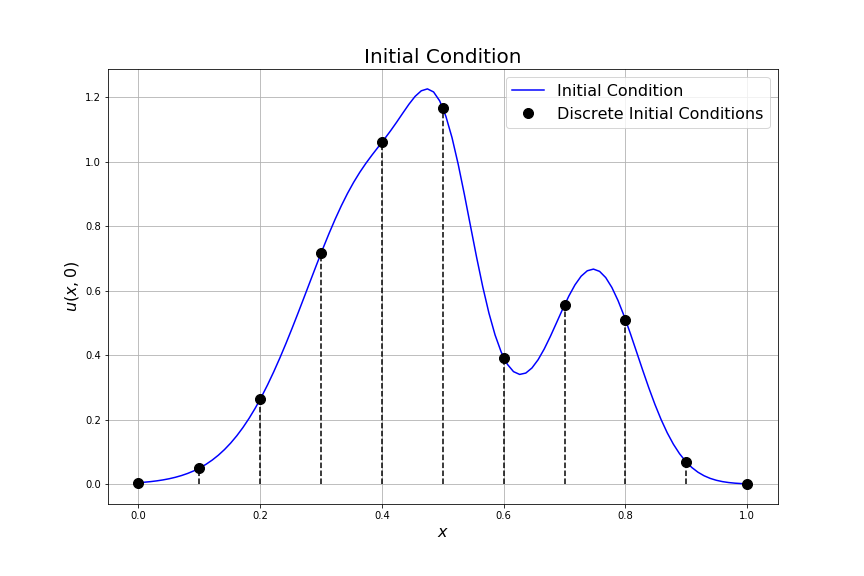
Figure C.1: An initial condition for the heat equation.
When solving this PDE numerically in the past we typically discretized both the spatial and the time derivative and then looped over time to build the solutions. However, there is an alternative way to proceed. If we first discretize the spatial derivative and not the time derivative then we will end up with a system of ordinary differential equations – one for each point in the spatial discretization.
Let’s make this more clear with a concrete example. Say we partition the interval \([0,1]\) into 10 equal sub intervals using 11 points, \(x_0 = 0, x_1 = 0.1, x_2 = 0.2, \ldots, x_{11} = 1\). If we only discretize the spatial derivative \(u_{xx}\) and, for the time being, leave the time derivatives alone we get the system of approximations \[\begin{eqnarray} u(x_0,t) &=& 0 \quad \text{(left boundary condition)} \\ \frac{\partial u(t,x_1)}{\partial t} &\approx& D\frac{u(t,x_0) - 2u(t,x_1) + u(t,x_2)}{\Delta x^2} \\ \frac{\partial u(t,x_2)}{\partial t} &\approx& D\frac{u(t,x_1) - 2u(t,x_2) + u(t,x_3)}{\Delta x^2} \\ \vdots \qquad && \qquad \qquad \qquad \vdots \\ \frac{\partial u(t,x_{9})}{\partial t} &\approx& D\frac{u(t,x_8) - 2u(t,x_{9}) + u(t,x_{10})}{\Delta x^2} \\ u(x_{10},t) &=& 0 \quad \text{(right boundary condition)} \end{eqnarray}\] where \(\Delta x = 0.1\) in this specific close. The value of \(x\) in each of the equations is fixed so we can view \(u(t,x_1)\) as a different function from \(u(t,x_2)\) which is different from \(u(t,x_3)\) and so on. In other words, if we let \(u_1 = u(t,x_1)\), \(u_2 = u(t,x_2)\), \(\ldots\), \(u(t,x_{9}) = u_{9}(t)\) we get the coupled system of ordinary differential equations \[\begin{eqnarray} \frac{\partial u_1}{\partial t} &=& D\frac{0 - 2u_1(t) + u_2(t)}{\Delta x^2} \\ \frac{\partial u_2}{\partial t} &=& D\frac{u_1(t) - 2u_2(t) + u_3(t)}{\Delta x^2} \\ \vdots \quad && \qquad \qquad \vdots \\ \frac{\partial u_{9}}{\partial t} &=& D\frac{u_8(t) - 2u_{9}(t) + 0}{\Delta x^2} \end{eqnarray}\] in the functions \(u_1, u_2, \ldots, u_{9}\).
The initial conditions for these ODEs are given by the initial condition function for the PDE shown as the black points in Figure C.1. One way to think of our new system is that the coupled ODEs track the lengths of the black dashed lines in Figure C.1 as they evolve in time. This technique is called the method of lines.
Now we have re-framed the problem of approximating the solution to the PDE as a problem of numerically solving a (potentially very large) system of ODEs. Thankfully we already know several tools for solving systems of ODEs. We just need to choose a method for stepping through time. Our choices, from Chapter 5, are Euler’s method, the Midpoint method, and the RK4 method. However, practitioners of numerical analysis typically lean on pre-built tools to do the job when using the method of lines. In the case of Python, there is a nice tool in the scipy library to do the time stepping which leverages a very powerful (RK4-like) method for doing the time stepping. You should stop now and check out Exercise 5.79, if you haven’t already, since it gives several of the details about how to use scipy.integrate.odeint().
Let’s put this into practice.
# import the proper libraries
import numpy as np
import matplotlib.pyplot as plt
from scipy.integrate import odeint # this one will do the time stepping

u0 = lambda x: ??? # define an appropriatet initial condition
x = np.linspace(0,1, ???) # choose a spatial grid
dx = ??? # calculate the value of Delta x
D = ??? # your value of the diffusion coefficient

# Now define a function for the spatial discretization
def F(u,t):
  dudt = np.zeros_like(u)
  dudt[0] = ??? # left Dirichley boundary condition
  dudt[-1] = ??? # right Dirichlet boundary condition
  # use vector smart computations to build all of the equations at once
  dudt[1:-1] = D*(u[???] - 2*u[???] + u[???] ) / dx**2
  return dudt

t = np.linspace(0,???,???) # build a spatial domain
dt = ??? # calculate Delta t

# Now build an array to store the time steps of the numerical solution
U = np.zeros( (len(t), len(x)) )
U[0,:] = u0(x) # put the initial condition in the correct row
The next small block of code will do all of the hard work of time stepping for us. Your first task is to explain completely what this small block of code does. You may want to refer to Exercise 5.79 and/or the help documentation for scipy.integrate.odeint.
for n in range(len(t)-1):
  U[n+1,:] = odeint(F, U[n,:], [0,dt])[1,:]
To complete this Exercise create several plots showing the time evolution of the solution. As an example, Figure C.2 shows several snapshots of the time evolution of the heat equation with the initial condition given in Figure C.1. In this simulation we use \(D = 0.2\) and \(\Delta t = 0.02\). Figure C.3 shows the same solution but were we use more spatial points to arrive at a smoother approximation. Experiment with the values of \(D\), \(\Delta x\), and \(\Delta t\) (and hence the ratio \(D \Delta t / \Delta x^2\)) to see if you can force the solution to become unstable.
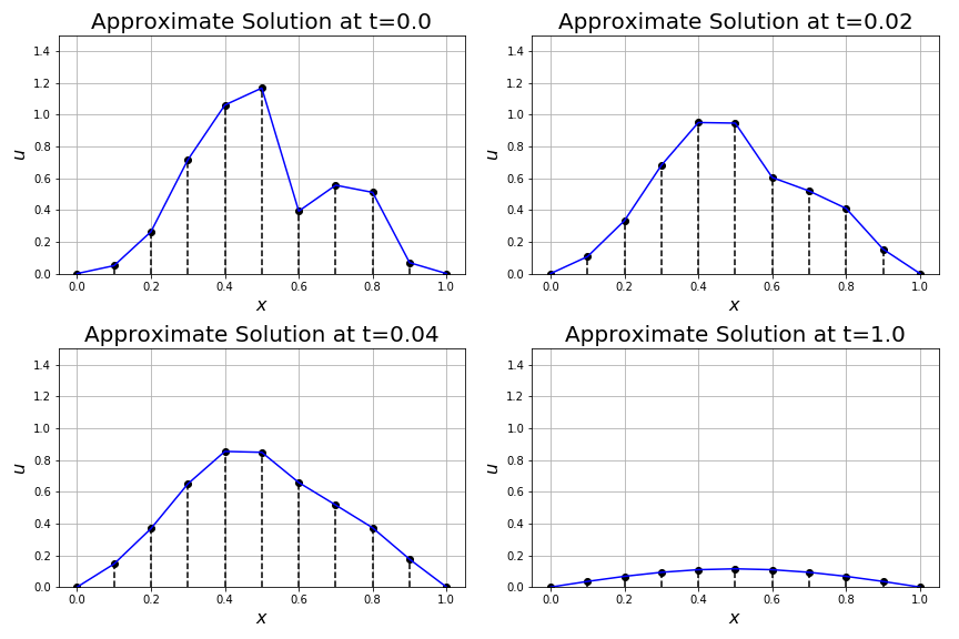
Figure C.2: A method of lines solution to the heat equation.
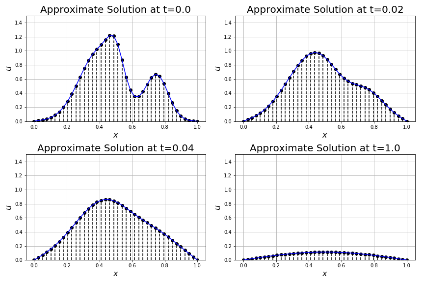
Figure C.3: A smoother method of lines solution to the heat equation.
Exercise C.24 We can use the method of lines approach to solving PDEs for the more than just the heat equation. Recall the traveling wave equation \[u_t + v u_x = 0\] where the parameter \(v\) is the speed of propogation of the traveling wave. Recall further that we had all sorts of trouble getting a stable numerical solution to this equation. Now would be a good time to refer back to the section and your work on the traveling wave equation.
Choose an appropriate initial condition and build a method of lines numerical solution to the traveling wave equation. Experiment with your solution and see if you get the same stability issues that we had with the traveling wave equation before. (Remember to choose your spatial derivative method wisely.)We haven’t yet mentioned using the method of lines for the wave equation, and that’s for a good reason. Recall that the 1D wave equation is \(u_{tt} = c u_{xx}\), and the fact that the time derivative is second order requires us to pay a bit closer attention – we can’t just naturally apply an ODE time stepper to a second order time derivative. In your ODE training you likely ran into second order ordinary differential equations in the context of harmonic oscillators. One technique for solving these types of ODEs was to introduce a new variable for the velocity of the oscillator and then to solve the resulting system of equations. We can do the same thing with PDEs.
Define the velocity function \(v = u_t\) and observe that the wave equation \(u_{tt} = cu_{xx}\) can now be written as \(v_t = cu_{xx}\). Hence we have the system of PDEs \[\begin{eqnarray} u_t &=& v \\ v_t &=& c u_{xx}. \end{eqnarray}\]
If we discretize the domain then at each point in the domain we have a value of the position, \(u\), and the velocity, \(v\). That is to say that we have twice as many differential equations to keep track of at each point in the spatial discretization, and this potentially causes some housekeeping headaches in your code. One way to manage this doubling of data is to take the even indexed entries of our solution vector to be \(u\) and to take the odd indexed entries to be \(v\). Thus, for each time step the numerical solution vector will be of the form \[[u_0, v_0, u_1, v_1, u_2, v_2, ...]\] where the subscripts correspond to the indices of the \(x\) coordinates. Hence, if we just want to extract the values of \(u\) we would take every other value starting at index 0. If we want to extract the values of \(v\) we would take every other value starting at index 1.
# start by importing the proper libraries
import numpy as np
import matplotlib.pyplot as plt
from scipy.integrate import odeint

# set up the spatial domain
x = np.linspace(0,1,???)
dx = ???

# set up the time domain
t = np.linspace(0,???,???)
dt = ???

# pick the stiffness parameter for the string
c = 2

# The input "uv" is the vector with u in the even indexed
# entries and v in the odd indexed entries.
def F(uv,t):
  duvdt = np.zeros_like(uv)
  duvdt[0] = ??? # left boundary position
  duvdt[1] = ??? # left boundary velocity
  duvdt[-2] = ??? # right boundary position
  duvdt[-1] = ??? # right boundary velocity
  # Next we need to build the equation u_t = v for
  # the interior points in the domain.
  duvdt[???:???:2] = uv[???:???:2]
  # Finally we need to build the equation v_t = c*u_xx for
  # the interion points in the domain.
  duvdt[???:???:2] = c*(uv[???:???:2]-2*uv[???:???:2]+uv[???:???:2])/dx**2
  return duvdt

u0 = ??? # pick an initial position
v0 = ??? # pick an initial velocity
# Set up storage for all of the time steps
UV = np.zeros( (len(t), 2*len(x)) ) # why are we doing 2*len(x)?
UV[0,???:???:2] = u0 # put the initial position in the right spot
UV[0,???:???:2] = v0 # put the initial velocity in the right spot

# Finally for the method of lines implementation.
for n in range(len(t)-1):
  UV[n+1,:] = odeint(F,UV[n,:],[0,dt])[1,:]
Plotting the solution is up to you. Just keep in mind that the position function \(u\) is in the even indexed columns of the array UV. If you wanted to plot the velocity of the string you now have the information too!
Exercise C.26 Using the method of lines and splitting the wave equation into a system of PDEs actually allows for a simpler implementation of non-trivial initial velocity functions. Pause and ponder here for a moment: we almost always took our initial velocity to be zero in all prior implementations. Why? Why are things easier now?
Experiment with numerically solving the 1D wave equation using several different initial positions and velocities. Moreover, modify your code to allow for different types of boundary conditions. Produce several snapshots of your more interesting simulations.Let’s return to the heat equation for a moment. In our implementations of the method of lines for the heat equation we made a second-order discretization in space of the form \[u_{xx} \approx \frac{u_{n+1} - 2u_n + u_{n-1}}{\Delta x^2}.\] In our implementation we coded this directly using carefully chosen indices. However, this is another way to build this discretization efficiently. Observe that at any time step we can produce the spatial discretization as a matrix-vector product as follows: \[\frac{D}{\Delta x^2}\begin{pmatrix} -2 & 1 & 0 & 0 & 0 & \cdots \\ 1 & -2 & 1 & 0 & 0 & \cdots \\ 0 & 1 & -2 & 1 & 0 & \cdots \\ \vdots & & & \ddots & & \end{pmatrix}\begin{pmatrix} u_1 \\ u_2 \\ u_3 \\ \vdots \end{pmatrix}\] Stop now and verify that the matrix-vector product will indeed produce the correct spatial discretization.
Using this new form of the spatial discretization we now can rewrite the PDE as a system of ODEs in the form \[\frac{\partial \boldsymbol{u}}{\partial t} = A \boldsymbol{u}\] where \(\boldsymbol{u} = \begin{pmatrix} u_1 & u_2 & u_3 & \cdots & u_{n-1} \end{pmatrix}^T\).
OK. This is all well and good, but there was nothing really wrong with the way that we implemented the spatial derivative in the past. Let’s recall a theorem from differential equations.
Using this theorem we now have a way to solve the associated time-dependent system of ODEs exactly! That’s right! We can avoid the use of any time stepping routine all together by just remembering some linear algebra (… ahhh linear algebra).
Exercise C.28 Write code to solve the 1D heat equation with a second order spatial discretization and an exact solution to the resulting system of ODEs. There is no time stepping needed, but instead your code will need to leverage some linear algebra.
Hint: Usenp.linalg.eig to find the eigenvalues and eigenvectors for you.