3 Calculus
3.1 Intro to Numerical Calculus
The calculus was the first achievement of modern mathematics and it is difficult to overestimate its importance.
–Hungarian-American Mathematician John von Neumann
In this chapter we build some of the common techniques for approximating the two primary computations in calculus: taking derivatives and evaluating definite integrals. Beyond differentiation and integration one of the major applications of differential calculus was optimization. The last several sections of this chapter focus on numerical routines for approximating the solutions to optimization problems. To see an introduction video for this chapter go to https://youtu.be/58zrgdf1cdY.
Recall the typical techniques from differential calculus: the power rule, the chain rule, the product rule, the quotient rule, the differentiation rules for exponentials, inverses, and trig functions, implicit differentiation, etc. With these rules, and enough time and patience, we can find a derivative of any algebraically defined function. The truth of the matter is that not all functions are given to us algebraically, and even the ones that are given algebraically are sometimes really cumbersome.
Exercise 3.2 When a police officer fires a radar gun at a moving car it uses a laser to measure the distance from the officer to the car:
The speed of light is constant.
The time between when the laser is fired and when the light reflected off of the car is received can be measured very accurately.
Using the formula \(\text{distance} = \text{rate} \cdot \text{time}\), the time for the laser pulse to be sent and received can then be converted to a distance.
Integration, on the other hand, is a more difficult situation. You may recall some of the techniques of integral calculus such as the power rule, \(u\)-substitution, and integration by parts. However, these tools are not enough to find an antiderviative for any given function. Furthermore, not every function can be written algebraically.
What you’ve seen here are just a few examples of why you might need to use numerical calculus instead of the classical routines that you learned earlier in your mathematical career. Another typical need for numerical derivatives and integrals arises when we approximate the solutions to differential equations in the later chapters of this book.
Throughout this chapter we will make heavy use of Taylor’s Theorem to build approximations of derivatives and integrals. If you find yourself still a bit shaky on Taylor’s Theorem it would probably be wise to go back to Section 1.4 and do a quick review.
At the end of the chapter we’ll examine a numerical technique for solving optimization problems without explicitly finding derivatives. Then we’ll look at a common use of numerical calculus for fitting curves to data.
3.2 Differentiation
3.2.1 The First Derivative
Exercise 3.6 Recall from your first-semester Calculus class that the derivative of a function \(f(x)\) is defined as \[f'(x) = \lim_{\Delta x \to 0} \frac{f(x+\Delta x) - f(x)}{\Delta x}\] A Calculus student proposes that it would just be much easier if we dropped the limit and instead just always choose \(\Delta x\) to be some small number, like \(0.001\) or \(10^{-6}\). Discuss the following questions:
When might the Calculus student’s proposal actually work pretty well in place of calculating an actual derivative?
When might the Calculus student’s proposal fail in terms of approximating the derivative?
In this section we’ll build several approximation of first and second derivatives. The primary idea for each of these approximations is:
- Partition the interval \([a,b]\) into \(N\) sub intervals
- Define the distance between two points in the partition as \(h\).
- Approximate the derivative at any point \(x\) in the interval \([a,b]\) by using linear combinations of \(f(x-h)\), \(f(x)\), \(f(x+h)\), and/or other points in the partition.
Partitioning the interval into discrete points turns the continuous problem of finding a derivative at every real point in \([a,b]\) into a discrete problem where we calculate the approximate derivative at finitely many points in \([a,b]\).
![A partition of the interval $[a,b]$.](images/Ch03_IntervalPartition.png)
Figure 3.1: A partition of the interval \([a,b]\).
Figure 3.1 shows a depiction of the partition as well as making clear that \(h\) is the separation between each of the points in the partition. Note that in general the points in the partition do not need to be equally spaced, but that is the simplest place to start.
Exercise 3.7 Let’s take a close look at partitions before moving on to more details about numerical differentiation.
- If we partition the interval \([0,1]\) into \(3\) equal sub intervals each with length \(h\) then:
- \(h = \underline{\hspace{1in}}\)
- \([0,1] = [0,\underline{\hspace{0.25in}}] \cup [\underline{\hspace{0.25in}},\underline{\hspace{0.25in}}] \cup [\underline{\hspace{0.25in}},1]\)
- There are four total points that define the partition. They are \(0, ??, ??, 1\).
- If we partition the interval \([3,7]\) into \(5\) equal sub intervals each with length \(h\) then:
- \(h = \underline{\hspace{1in}}\)
- \([3,7] = [3,\underline{\hspace{0.25in}}] \cup [\underline{\hspace{0.25in}},\underline{\hspace{0.25in}}] \cup [\underline{\hspace{0.25in}},\underline{\hspace{0.25in}}] \cup [\underline{\hspace{0.25in}},\underline{\hspace{0.25in}}] \cup [\underline{\hspace{0.25in}},7]\)
- There are 6 total points that define the partition. They are \(0, ??, ??, ??, ??, 7\).
- More generally, if a closed interval \([a,b]\) contains \(N\) equal sub intervals where \[ [a,b] = \underbrace{[a,a+h] \cup [a+h, a+2h] \cup \cdots \cup [b-2h,b-h] \cup [b-h,b]}_{\text{$N$ total sub intervals}} \] then the length of each sub interval, \(h\), is given by the formula \[ h = \frac{?? - ??}{??}. \]
numpy library there is a nice tool called np.linspace() that partitions an interval in exactly the way that we want. The command takes the form np.linspace(a, b, n) where the interval is \([a,b]\) and \(n\) the number of points used to create the partition. For example, np.linspace(0,1,5) will produce the list of numbers 0, 0.25, 0.5, 0.75, 1. Notice that there are 5 total points, the first point is \(a\), the last point is \(b\), and there are \(n-1\) total sub intervals in the partition. Hence, if we want to partition the interval \([0,1]\) into 20 equal sub intervals then we would use the command np.linspace(0,1,21) which would result in a list of numbers starting with 0, 0.05, 0.1, 0.15, etc. What command would you use to partition the interval \([5,10]\) into \(100\) equal sub intervals?
Exercise 3.9 Consider the Python command np.linspace(0,1,50).
- What interval does this command partition?
- How many points are going to be returned?
- How many equal length subintervals will we have in the resulting partition?
- What is the length of each of the subintervals in the resulting partition?
Now let’s get back to the discussion of numerical differentiation. If we recall that the definition of the first derivative of a function is \[ \begin{aligned} \frac{df}{dx} = \lim_{h \to 0} \frac{f(x+h) - f(x)}{h}. \label{eqn:derivative_defintiion}\end{aligned}\] our first approximation for the first derivative is naturally \[ \begin{aligned} \frac{df}{dx} \approx \frac{f(x+h) - f(x)}{h}. \label{eqn:derivative_first_approx}\end{aligned}\] In this approximation of the derivative we have simply removed the limit and instead approximated the derivative as the slope. It should be clear that this approximation is only good if \(h\) is small. In Figure 3.2 we see a graphical depiction of what we’re doing to approximate the derivative. The slope of the tangent line (\(\Delta y / \Delta x\)) is what we’re after, and a way to approximate it is to calculate the slope of the secant line formed by looking \(h\) units forward from the point \(x\).
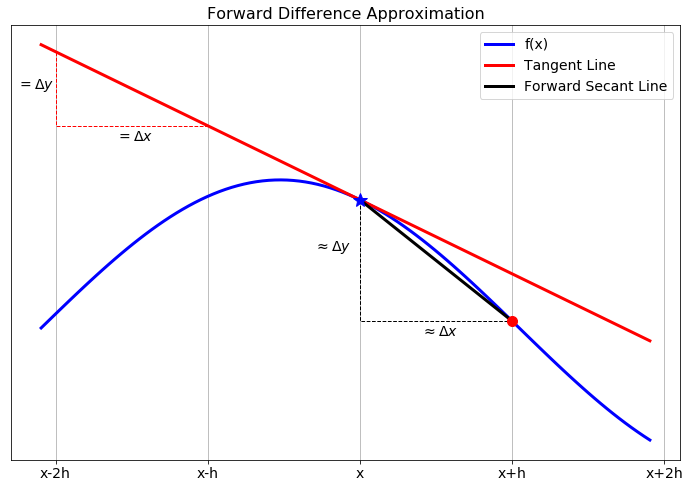
Figure 3.2: The forward difference differentiation scheme for the first derivative.
While this is the simplest and most obvious approximation for the first derivative there is a much more elegant technique, using Taylor series, for arriving at this approximation. Furthermore, the Taylor series technique suggests an infinite family of other techniques.
Exercise 3.12 In the formula that you developed in Exercise 3.11, if we were to drop everything after the fraction (called the remainder) we know that we would be introducing error into our derivative computation. If \(h\) is taken to be very small then the first term in the remainder is the largest and everything else in the remainder can be ignored (since all subsequent terms should be extremely small … pause and ponder this fact). Therefore, the amount of error we make in the derivative computation by dropping the remainder depends on the power of \(h\) in that first term in the remainder.
What is the power of \(h\) in the first term of the remainder from Exercise 3.11?Definition 3.1 (Order of a Numerical Differentiation Scheme) The order of a numerical derivative is the power of the step size in the first term of the remainder of the rearranged Taylor Series. For example, a first order method will have “\(h^1\)” in the first term of the remainder. A second order method will have “\(h^2\)” in the first term of the remainder. Etc.
The error that you make by dropping the remainder is proportional to the power of \(h\) in the first term of the remainder. Hence, the order of a numerical differentiation scheme tells you how to quantify the amount of error that you are making by using that approximation scheme.Definition 3.2 (Big O Notation) We say that the error in a differentiation scheme is \(\mathcal{O}(h)\) (read: “big O of \(h\)”), if and only if there is a positive constant \(M\) such that \[ |Error| \le M \cdot h.\] This is equivalent to saying that a differentiation method is “first order.” In other words, if the error in a numerical differentiation scheme is proportional to the length of the subinterval in the partition of the interval (see Figure 3.1) then we call that scheme “first order” and say that the error is \(\mathcal{O}(h)\).
More generally, we say that the error in a differentiation scheme is \(\mathcal{O}(h^k)\) (read: “big O of \(h^k\)”) if and only if there is a positive constant \(M\) such that \[ |Error| \leq M \cdot h^k. \] This is equivalent to saying that a differentiation scheme is “\(k^{th}\) order.” This means that the error in using the scheme is proportional to \(h^k\).Theorem 3.1 In problem 3.11 we derived a first order approximation of the first derivative: \[ f'(x) = \frac{f(x+h) - f(x)}{h} + \mathcal{O}(h).\] In this formula, \(h = \Delta x\) is the step size.
If we approximate the first derivative of a differentiable function \(f(x)\) at the point \(x\) with the formula \[ f'(x) \approx \frac{f(x+h)-f(x)}{h} \] then we know that the error in this approximation is proprotional to \(h\) since the approximation scheme is \(\mathcal{O}(h)\).3.2.2 Error Analysis
Exercise 3.13 Consider the function \(f(x) = \sin(x) (1- x)\). The goal of this problem is to make sense of the discussion of the “order” of the derivative approximation. You may want to pause first and reread the previous couple of pages.
Find \(f'(x)\) by hand.
Use your answer to part (a) to verify that \(f'(1) = -\sin(1) \approx -0.8414709848\).
To approximate the first derivative at \(x=1\) numerically with our first order approximation formula from Theorem 3.1 we calculate \[ f'(1) \approx \frac{f(1+h) - f(1)}{h}.\] We want to see how the error in the approximation behaves as \(h\) is made smaller and smaller. Fill in the table below with the derivative approximation and the absolute error associated with each given \(h\). You may want to use a spreadsheet to organize your data (be sure that you’re working in radians!).
\(h\) Approx. of \(f'(1)\) Exact value of \(f'(1)\) Abs. % Error \(2^{-1} = 0.5\) \(\frac{f(1+0.5)-f(1)}{0.5} \approx -0.99749\) \(-\sin(1) \approx -0.841471\) \(18.54181\%\) \(2^{-2} = 0.25\) \(\frac{f(1+0.25)-f(1)}{0.25} \approx -0.94898\) \(-\sin(1) \approx -0.841471\) \(12.77687\%\) \(2^{-3} = 0.125\) \(-\sin(1)\) \(2^{-4}=0.0625\) \(-\sin(1)\) \(2^{-5}\) \(-\sin(1)\) \(2^{-6}\) \(-\sin(1)\) \(2^{-7}\) \(-\sin(1)\) \(2^{-8}\) \(-\sin(1)\) \(2^{-9}\) \(-\sin(1)\) \(2^{-10}\) \(-\sin(1)\) There was nothing really special in part (c) about powers of 2. Use your spreadsheet to build similar tables for the following sequences of \(h\): \[\begin{aligned} h &= 3^{-1}, \, 3^{-2}, \, 3^{-3}, \, \ldots \\ h &= 5^{-1}, \, 5^{-2}, \, 5^{-3}, \, \ldots \\ h &= 10^{-1}, \, 10^{-2}, \, 10^{-3}, \, \ldots \\ h &= \pi^{-1}, \, \pi^{-2}, \, \pi^{-3}, \, \ldots \\ \end{aligned}\]
Observation: If you calculate a numerical derivative with a forward difference and then calculate the absolute percent error with a fixed value of \(h\), then what do you expect to happen to the absolute error if you divide the value of \(h\) by some positive contant \(M\)? It may be helpful at this point to go back to your table and include a column called the error reduction factor where you find the ratio of two successive absolute percenter errors. Observe what happens to this error reduction factor as \(h\) gets smaller and smaller.
What does your answer to part (e) have to do with the approximation order of the numerical derivative method that you used?
Exercise 3.14 The following incomplete block of Python code will help to streamline the previous problem so that you don’t need to do the computation with a spreadsheet.
- Comment every existing line with a thorough description.
- Fill in the blanks in the code to perform the spreadsheet computations from the previous problem.
- Run the code for several forms of \(h\)
- Do you still observe the same result that you observed in part (e) of the previous problem?
- We know that for \(h \to 0\) the derivative approximation should mathematically tend toward the exact derivative. Modify the code slightly to see if this is the case. Explain what you see.
import numpy as np
import matplotlib.pyplot as plt
f = lambda x: np.sin(x) * (1-x) # what does this line do?
exact = -np.sin(1) # what does this line do?
H = 2.0**(-np.arange(1,10)) # what does this line do?
AbsPctError = [] # start off with a blank list of errors
for h in H:
    approx = # FINISH THIS LINE OF CODE
    AbsPctError.append( np.abs( (approx - exact)/exact ) )
    if h==H[0]:
      print("h=",h,"\t Absolute Pct Error=", AbsPctError[-1])
    else:
      err_reduction_factor = AbsPctError[-2]/AbsPctError[-1]
      print("h=",h,"\t Absolute Pct Error=", AbsPctError[-1],
              "with error reduction",err_reduction_factor)
plt.loglog(H,AbsPctError,'b-*') # Why are we build a loglog plot?
plt.grid()
plt.show()
Exercise 3.15 Assume that \(f(x)\) is some differentiable function and that we have calculated the value of \(f'(c)\) using the forward difference formula \[f'(c) \approx \frac{f(c+h) - f(c)}{h}.\] Using what you learned from the previous problem to fill in the following table.
| My \(h\) | Absolute Percent Error |
|---|---|
| \(0.2\) | \(2.83\%\) |
| \(0.1\) | |
| \(0.05\) | |
| \(0.02\) |
3.2.3 Efficient Coding
Now that we have a handle on how the first order approximation scheme for the first derivative works and how the errors will propagate, let’s build some code that will take in a function and output the approximate first derivative on an entire interval instead of just at a single point.
Exercise 3.17 We want to build a Python function that accepts:
- a mathematical function,
- the bounds of an interval,
- and the number of subintervals.
The function will return a first order approximation of the first derivative at every point in the interval except at the right-hand side. For example, we could send the function \(f(x) = \sin(x)\), the interval \([0,2\pi]\), and tell it to split the interval into 100 subintervals. We would then get back a value of the derivative \(f'(x)\) at all of the points except at \(x=2\pi\).
- First of all, why can’t we compute a derivative at the last point?
- Next, fill in the blanks in the partially complete code below. Every line needs to have a comment explaining exactly what it does.
import numpy as np
import matplotlib.pyplot as plt
def FirstDeriv(f,a,b,N):
    x = np.linspace(a,b,N+1) # What does this line of code do?
    # What's up with the N+1 in the previous line?
    h = x[1] - x[0] # What does this line of code do?
    df = [] # What does this line of code do?
    for j in np.arange(len(x)-1): # What does this line of code do?
        # What's up with the -1 in the definition of the loop?
        #
        # Now we want to build the approximation
        # (f(x+h) - f(x)) / h.
        # Obviously "x+h" is just the next item in the list of
        # x values so when we do f(x+h) mathematically we should
        # write f( x[j+1] ) in Python (explain this).
        # Fill in the question marks below
        df.append( (f( ??? ) - f( ??? )) / h )
return df- Now we want to call upon this function to build the first order approximation of the first derivative for some function. We’ll use the function \(f(x) = \sin(x)\) on the interval \([0,2\pi]\) with 100 sub intervals (since we know what the answer should be). Complete the code below to call upon your
FirstDeriv()function and to plot \(f(x)\), \(f'(x)\), and the approximation of \(f'(x)\).
f = lambda x: np.sin(x)
exact_df = lambda x: np.cos(x)
a = ???
b = ???
N = 100 # What is this?
x = np.linspace(a,b,N+1)
# What does the prevoius line do?
# What's up with the N+1?

df = FirstDeriv(f,a,b,N) # What does this line do?

# In the next line we plot three curves:
# 1) the function f(x) = sin(x)
# 2) the function f'(x) = cos(x)
# 3) the approximation of f'(x)
# However, we do something funny with the x in the last plot. Why?
plt.plot(x,f(x),'b',x,exact_df(x),'r--',x[0:-1], df, 'k-.')
plt.grid()
plt.legend(['f(x) = sin(x)',
            'exact first deriv',
            'approx first deriv'])
plt.show()- Implement your completed code and then test it in several ways:
- Test your code on functions where you know the derivative. Be sure that you get the plots that you expect.
- Test your code with a very large number of sub intervals, \(N\). What do you observe?
- Test your code with small number of sub intervals, \(N\). What do you observe?
numpy lists in Python. Instead of looping over all of the elements we can take advantage of the fact that every thing is stored in lists. Hence we can just do list operations and do all of the subtractions and divisions at once without a loop.
- From your previous code, comment out the following lines.
#     df = []
#     for j in np.arange(len(x)-1):
# df.append( (f(x[j+1]) - f(x[j])) / h )- From the line of code
x = np.linspace(a,b,N+1)we build a list of \(N+1\) values of \(x\) starting at \(a\) and ending at \(b\). In the following questions remember that Python indexes all lists starting at 0. Also remember that you can call on the last element of a list using an index of-1. Finally, remember that if you dox[p:q]in Python you will get a list ofxvalues starting at indexpand ending at indexq-1.- What will we get if we evaluate the code
x[1:]? - What will we get if we evaluate the code
f(x[1:])? - What will we get if we evaluate the code
x[0:-1]?
- What will we get if we evaluate the code
f(x[0:-1])? - What will we give if we evaluate the code
f(x[1:]) - f(x[0:-1])? - What will we give if we evaluate the code
( f(x[1:]) - f(x[0:-1]) ) / h?
- What will we get if we evaluate the code
- Replace the lines that you commented out in part (a) of this exercise with the appropriate single line of code that builds all of the approximations for the first derivative all at once without the need for a loop. What you did in part (b) should help. Your simplified first order first derivative function should look like the code below.
def FirstDeriv(f,a,b,N):
    x = np.linspace(a,b,N+1)
    h = x[1] - x[0]
    df = # your line of code goes here?
    return df
Exercise 3.19 Write code that finds a first order approximation for the first derivative of \(f(x) = \sin(x) - x\sin(x)\) on the interval \(x \in (0,15)\). Your script should output two plots (side-by-side).
- The left-hand plot should show the function in blue and the approximate first derivative as a red dashed curve. Sample code for this problem is given below.
import matplotlib.pyplot as plt
import numpy as np

f = lambda x: np.sin(x) - x*np.sin(x)
a = 0
b = 15
N = # make this an appropriately sized number of subintervals
x = np.linspace(a,b,N+1) # what does this line do?
y = f(x) # what does this line do?
df = FirstDerivFirstOrder(f,a,b,N) # what does this line do?

fig, ax = plt.subplots(1,2) # what does this line do?
ax[0].plot(x,y,'b',x[0:-1],df,'r--') # what does this line do?
ax[0].grid()- The right-hand plot should show the absolute error between the exact derivative and the numerical derivative. You should use a logarithmic \(y\) axis for this plot.
exact = lambda x: # write a function for the exact derivative
# There is a lot going on the next line of code ... explain it.
ax[1].semilogy(x[0:-1],abs(exact(x[0:-1]) - df))
ax[1].grid()- Play with the number of sub intervals, \(N\), and demonstrate the fact that we are using a first order method to approximate the first derivative.
3.2.4 A Better First Derivative
Next we’ll build a more accurate numerical first derivative scheme. The derivation technique is the same: play a little algebra game with the Taylor series and see if you can get the first derivative to simplify out. This time we’ll be hoping to have a better error approximation.
Exercise 3.20 Consider again the Taylor series for an infinitely differentiable function \(f(x)\): \[ f(x) = f(x_0) + \frac{f'(x_0)}{1!} (x-x_0)^1 + \frac{f''(x_0)}{2!}(x-x_0)^2 + \frac{f^{(3)}(x_0)}{3!}(x-x_0)^3 + \cdots \]
Replace the “\(x\)” in the Taylor Series with “\(x+h\)” and replace the “\(x_0\)” in the Taylor Series with “\(x\)” and simplify. \[f(x+h) = \underline{\hspace{3in}}\]
Now replace the “\(x\)” in the Taylor Series with “\(x-h\)” and replace the “\(x_0\)” in the Taylor Series with “\(x\)” and simplify. \[f(x-h) = \underline{\hspace{3in}}\]
Find the difference between \(f(x+h)\) and \(f(x-h)\) and simplify. Be very careful of your signs. \[f(x+h) - f(x-h) = \underline{\hspace{3in}}\]
Solve for \(f'(x)\) in your result from part (c). Fill in the question marks and blanks below once you have finished simplifying. \[f'(x) = \frac{??? - ???}{2h} + \underline{\hspace{3in}}.\]
Use your result from part (d) to verify that \[f'(x) = \underline{\hspace{2in}} + \mathcal{O}(h^2).\]
Draw a picture similar to Figure 3.2 showing what this scheme is doing graphically.
Exercise 3.21 Let’s return to the function \(f(x) = \sin(x)(1- x)\) but this time we will approximate the first derivative at \(x=1\) using the formula \[f'(1) \approx \frac{f(1+h) - f(1-h)}{2h}.\] You should already have the first derivative and the exact answer from Exercise 3.13 (if not, then go get them by hand again).
Fill in the table below with the derivative approximation and the absolute error associated with each given \(h\). You may want to use a spreadsheet to organize your data (be sure that you’re working in radians!).
\(h\) Approx. of \(f'(1)\) Exact value of \(f'(1)\) Abs. % Error \(2^{-3} = 0.5\) \(-\sin(1)\) \(2^{-3} = 0.25\) \(-\sin(1)\) \(2^{-3} = 0.125\) \(-\sin(1)\) \(2^{-4}=0.0625\) \(-\sin(1)\) \(2^{-5}\) \(-\sin(1)\) \(2^{-6}\) \(-\sin(1)\) \(2^{-7}\) \(-\sin(1)\) \(2^{-8}\) \(-\sin(1)\) \(2^{-9}\) \(-\sin(1)\) There was nothing really special in part (c) about powers of 2. Use your spreadsheet to build similar tables for the following sequences of \(h\): \[\begin{aligned} h &= 3^{-1}, \, 3^{-2}, \, 3^{-3}, \, \ldots \\ h &= 5^{-1}, \, 5^{-2}, \, 5^{-3}, \, \ldots \\ h &= 10^{-1}, \, 10^{-2}, \, 10^{-3}, \, \ldots \\ h &= \pi^{-1}, \, \pi^{-2}, \, \pi^{-3}, \, \ldots \end{aligned}\]
Observation: If you calculate a numerical derivative with a centered difference and calculate the resulting absolute percent error with a fixed value of \(h\), then what do you expect to happen to the absolute percent error if you divide the value of \(h\) by some positive constant \(M\)? It may be helpful to include a column in your table that tracks the error reduction factor as we decrease \(h\).
What does your answer to part (e) have to do with the approximation order of the numerical derivative method that you used?
Exercise 3.22 Assume that \(f(x)\) is some differentiable function and that we have calculated the value of \(f'(c)\) using the centered difference formula \[f'(c) \approx \frac{f(c+h) - f(c-h)}{2h}.\] Using what you learned from the previous problem to fill in the following table.
| My \(h\) | Absolute Percent Error |
|---|---|
| \(0.2\) | \(2.83\%\) |
| \(0.1\) | |
| \(0.05\) | |
| \(0.02\) | |
| \(0.002\) |
Exercise 3.25 The plot shown in Figure 3.3 shows the maximum absolute error between the exact first derivative of a function \(f(x)\) and a numerical first derivative approximation scheme. At this point we know two schemes: \[ f'(x) = \frac{f(x+h) - f(x)}{h} + \mathcal{O}(h) \] and \[ f'(x) = \frac{f(x+h) - f(x-h)}{2h} + \mathcal{O}(h^2). \]
- Which curve in the plot matches with which method. How do you know?
- Recreate the plot with a function of your choosing.
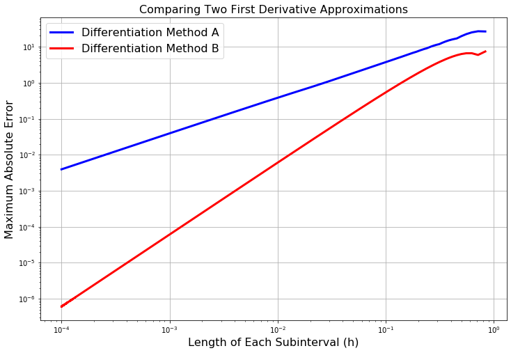
Figure 3.3: Maximum absolute error between the first derivative and two different approximations of the first derivative.
3.2.5 The Second Derivative
Now we’ll search for an approximation of the second derivative. Again, the game will be the same: experiment with the Taylor series and some algebra with an eye toward getting the second derivative to pop out cleanly. This time we’ll do the algebra in such a way that the first derivative cancels.
From the previous problems you already have Taylor expansions of the form \(f(x+h)\) and \(f(x-h)\). Let’s summarize them here since you’re going to need them for future computations. \[ \begin{aligned} f(x+h) &= f(x) + \frac{f'(x)}{1!} h + \frac{f''(x)}{2!} h^2 + \frac{f^{(3)}(x)}{3!} h^3 + \cdots \\ f(x-h) &= f(x) - \frac{f'(x)}{1!} h + \frac{f''(x)}{2!} h^2 - \frac{f^{(3)}(x)}{3!} h^3 + \cdots \end{aligned} \]
Exercise 3.26 The goal of this problem is to use the Taylor series for \(f(x+h)\) and \(f(x-h)\) to arrive at an approximation scheme for the second derivative \(f''(x)\).
Add the Taylor series for \(f(x+h)\) and \(f(x-h)\) and combine all like terms. You should notice that several terms cancel. \[f(x+h) + f(x-h) = \underline{\hspace{3in}}.\]
Solve your answer in part (a) for \(f''(x)\). \[f''(x) = \frac{?? - 2 \cdot ?? + ??}{h^2} + \underline{\hspace{1in}}.\]
If we were to drop all of the terms after the fraction on the right-hand side of the previous result we would be introducing some error into the derivative computation. What does this tell us about the order of the error for the second derivative approximation scheme we just built?
Exercise 3.27 Again consider the function \(f(x) = \sin(x)(1 - x)\).
Calculate the derivative of this function and calculate the exact value of \(f''(1)\).
If we calcuate the second derivative with the central difference scheme that you built in the previous exericse using \(h = 0.5\) then we get a 4.115% error. Stop now and verify this percent error calculation.
Based on our previous work with the order of the error in a numerical differentiation scheme, what do you predict the error will be if we calculate \(f''(1)\) with \(h = 0.25\)? With \(h = 0.05\)? With \(h = 0.005\)? Defend your answers.
Exercise 3.29 Test your second derivative code on the function \(f(x) = \sin(x) - x\sin(x)\) by doing the following.
Find the analytic second derivative by hand.
Find the numerical second derivative with the code that you just wrote.
Find the absolute difference between your numerical second derivative and the actual second derivative. This is point-by-point subtraction so you should end up with a vector of errors.
Find the maximum of your errors.
Now we want to see how the code works if you change the number of points used. Build a plot showing the value of \(h\) on the horizontal axis and the maximum error on the vertical axis. You will need to write a loop that gets the error for many different values of \(h\). Finally, it is probably best to build this plot on a log-log scale.
Discuss what you see? How do you see the fact that the numerical second derivative is second order accurate?
The table below summarizes the formulas that we have for derivatives thus far. The exercises at the end of this chapter contain several more derivative approximations. We will return to this idea when we study numerical differential equations in Chapter 5.
| Derivative | Formula | Error | Name |
|---|---|---|---|
| \(1^{st}\) | \(f'(x) \approx \frac{f(x+h) - f(x)}{h}\) | \(\mathcal{O}(h)\) | Forward Difference |
| \(1^{st}\) | \(f'(x) \approx \frac{f(x) - f(x-h)}{h}\) | \(\mathcal{O}(h)\) | Backward Difference |
| \(1^{st}\) | \(f'(x) \approx \frac{f(x+h) - f(x-h)}{2h}\) | \(\mathcal{O}(h^2)\) | Centered Difference |
| \(2^{nd}\) | \(f''(x) \approx \frac{f(x+h) - 2f(x) + f(x-h)}{h^2}\) | \(\mathcal{O}(h^2)\) | Centered Difference |
Exercise 3.30 Let \(f(x)\) be a twice differentiable function. We are interested in the first and second derivative of the function \(f\) at the point \(x = 1.74\). Use what you have learned in this section to answer the following questions. (For clarity, you can think of “\(f\)” as a different function in each of the following questions …it doesn’t really matter exactly what function \(f\) is.)
Johnny used a numerical first derivative scheme with \(h = 0.1\) to approximate \(f'(1.74)\) and found an abolute percent error of 3.28%. He then used \(h=0.01\) and found an absolute percent error of 0.328%. What was the order of the error in his first derivative scheme? How can you tell?
Betty used a numerical first derivative scheme with \(h = 0.2\) to approximate \(f'(1.74)\) and found an absolute percent error of 4.32%. She then used \(h=0.1\) and found an absolute percent error of 1.08%. What numerical first derivative scheme did she likely use?
Shelby did the computation \[f'(1.74) \approx \frac{f(1.78) - f(1.74)}{0.04}\] and found an absolute percent error of 2.93%. If she now computes \[f'(1.74) \approx \frac{f(1.75) - f(1.74)}{0.01}\] what will the new absolute percent error be?
Harry wants to compute \(f''(1.74)\) to within 1% using a central difference scheme. He tries \(h=0.25\) and gets an absolute percent error of 3.71%. What \(h\) should he try next so that his absolute percent error is less than (but close to) 1%?
3.3 Integration
Now we begin our work on the second principle computation of Calculus: evaluating a definite integral. Remember that a single-variable definite integral can be interpreted as the signed area between the curve and the \(x\) axis. In this section we will study three different techniques for approximating the value of a definite integral.
Exercise 3.31 Consider the shaded area of the region under the function plotted in Figure 3.4 between \(x=0\) and \(x=2\).
- What rectangle with area 6 gives an upper bound for the area under the curve? Can you give a better upper bound?
- Why must the area under the curve be greater than 3?
- Is the area greater than 4? Why/Why not?
- Work with your partner to give an estimate of the area and provide an estimate for the amount of error that you’re making.
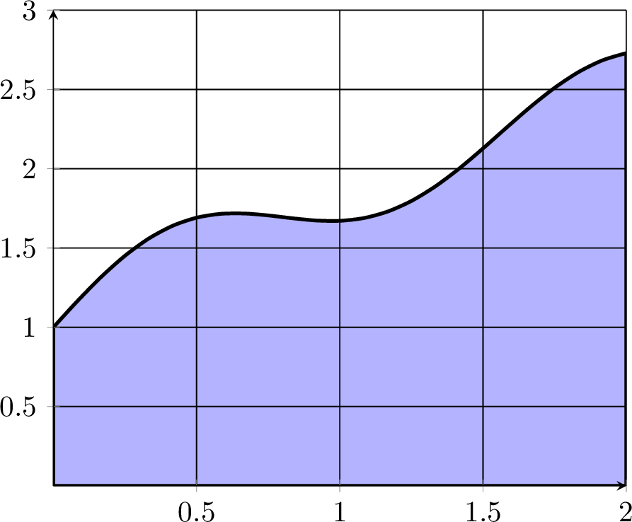
Figure 3.4: A sample integration
3.3.1 Riemann Sums
In this subsection we will build our first method for approximating definite integrals. Recall from Calculus that the definition of the Riemann integral is \[\begin{aligned} \int_a^b f(x) dx = \lim_{\Delta x \to 0} \sum_{j=1}^N f(x_j) \Delta x \label{eqn:Riemann_integral}\end{aligned}\] where \(N\) is the number of sub intervals on the interval \([a,b]\) and \(\Delta x\) is the width of the interval. As with differentiation, we can remove the limit and have a decent approximation of the integral so long as \(N\) is large (or equivalently, if \(\Delta x\) is small). \[\int_a^b f(x) dx \approx \sum_{j=1}^N f(x_j) \Delta x.\] You are likely familiar with this approximation of the integral from Calculus. The value of \(x_j\) can be chosen anywhere within the sub interval and three common choices are to use the left-aligned, the midpoint-aligned, and the right-aligned.
We see a depiction of this in Figure 3.5.
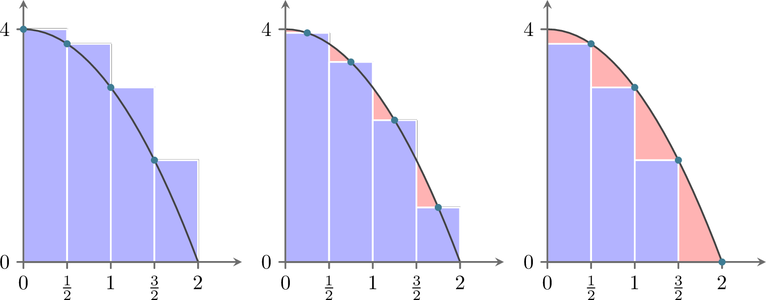
Figure 3.5: Left-aligned Riemann sums, midpoint-aligned Riemann sums, and right-aligned Riemann sums
Clearly, the more rectangles we choose the closer the sum of the areas of the rectangles will get to the integral.
left, right, or
midpoint rectangles. Test your code on several functions for which you know the integral. You
should write your code without any loops.
Exercise 3.33 Consider the function \(f(x) = \sin(x)\). We know the antiderivative for this function, \(F(x) = -\cos(x) + C\), but in this question we are going to get a sense of the order of the error when doing Riemann Sum integration.
Find the exact value of \[\int_0^{1} f(x) dx.\]
Now build a Riemann Sum approximation (using your code) with various values of \(\Delta x\). For all of your approximation use left-justified rectangles. Fill in the table with your results.
| \(\Delta x\) | Approx. Integral | Exact Integral | Abs. Percent Error |
|---|---|---|---|
| \(2^{-1} = 0.5\) | |||
| \(2^{-2} = 0.25\) | |||
| \(2^{-3}\) | |||
| \(2^{-4}\) | |||
| \(2^{-5}\) | |||
| \(2^{-6}\) | |||
| \(2^{-7}\) | |||
| \(2^{-8}\) |
There was nothing really special about powers of 2 in part (b) of this problem. Examine other sequences of \(\Delta x\) with a goal toward answering the question:
If we find an approximation of the integral with a fixed \(\Delta x\) and find an absolute percent error, then what would happen to the absolute percent error if we divide \(\Delta x\) by some positive constant \(M\)?What is the apparent approximation error of the Riemann Sum method using left-justified rectangles.
Theorem 3.2 In approximating the integral \(\int_a^b f(x) dx\) with a fixed interval width \(\Delta x\) we find an absolute percent error \(P\).
If we use left rectangles and an interval width of \(\frac{\Delta x}{M}\) then the absolute percent error will be approximately \(\underline{\hspace{1in}}\).
If we use right rectangles and an interval width of \(\frac{\Delta x}{M}\) then the absolute percent error will be approximately \(\underline{\hspace{1in}}\).
Exercise 3.35 The previous theorem could be stated in an equivalent way.
In approximating the integral \(\int_a^b f(x) dx\) with a fixed interval number of subintervals we find an absolute percent error \(P\).
If we use left rectangles and \(M\) times as many subintervals then the absolute percent error will be approximately \(\underline{\hspace{1in}}\).
If we use right rectangles and \(M\) times as many subintervals then the absolute percent error will be approximately \(\underline{\hspace{1in}}\).
3.3.2 Trapezoidal Rule
Now let’s turn our attention to some slightly better algorithms for calculating the value of a definite integral: The Trapezoidal Rule and Simpson’s Rule. There are many others, but in practice these two are relatively easy to implement and have reasonably good error approximations. To motivate the idea of the Trapezoid rule consider Figure 3.6. It is plain to see that trapezoids will make better approximations than rectangles at least in this particular case. Another way to think about using trapezoids, however, is to see the top side of the trapezoid as a secant line connecting two points on the curve. As \(\Delta x\) gets arbitrarily small, the secant lines become better and better approximations for tangent lines and are hence arbitrarily good approximations for the curve. For these reasons it seems like we should investigate how to systematically approximate definite integrals via trapezoids.
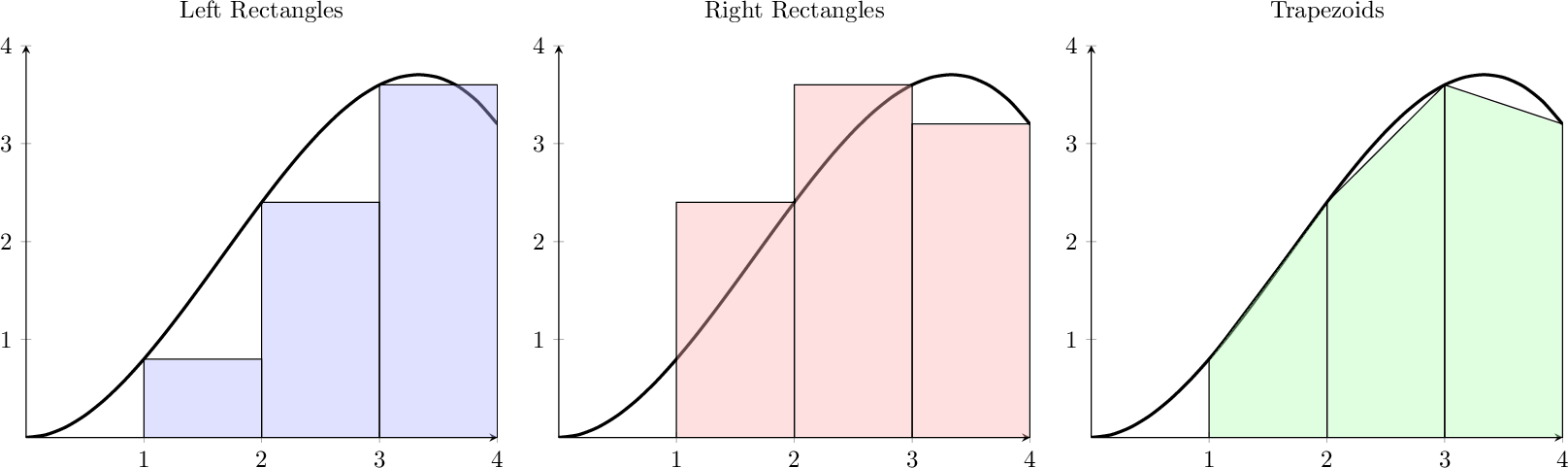
Figure 3.6: Motivation for using trapezoids to approximate a definite integral.
Exercise 3.37 Consider a single trapezoid approximating the area under a curve. From geometry we recall that the area of a trapezoid is \[A = \frac{1}{2}\left( b_1 + b_2 \right) h\] where \(b_1, b_2\) and \(h\) are marked in Figure 3.7. The function shown in the picture is \(f(x) = \frac{1}{5} x^2 (5-x)\). Find the area of the shaded region as an approximation to \[\int_1^4 \left( \frac{1}{5} x^2 (5-x) \right) dx.\]
Now use the same idea with \(h = \Delta x = 1\) from Figure 3.6 to approximate the area under the function \(f(x) = \frac{1}{5}x^2(5-x)\) between \(x=1\) and \(x=4\) using three trapezoids.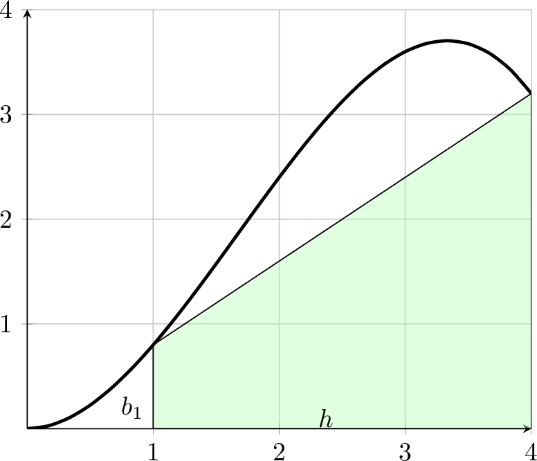
Figure 3.7: A single trapezoid to approximate area under a curve.
Exercise 3.38 Again consider the function \(f(x) = \frac{1}{5}x^2(5-x)\) on the interval \([1,4]\). We want to evaluate the integral \[\int_1^4 f(x) dx\] using trapezoids to approximate the area.
Work out the exact value of the definite integral by hand.
Summarize your answers to the previous problems in the following table then extend the data that you have for smaller and smaller values of \(\Delta x\).
| \(\Delta x\) | Approx. Integral | Exact Integral | Abs. % Error |
|---|---|---|---|
| \(3\) | |||
| \(1\) | |||
| \(1/3\) | |||
| \(1/9\) | |||
| \(\vdots\) | \(\vdots\) | \(\vdots\) | \(\vdots\) |
- From the table that you built in part (b), what do you conjecture is the order of the approximation error for the trapezoid method?
Definition 3.3 (The Trapezoidal Rule) We want to approximate \(\displaystyle \int_a^b f(x) dx\). One of the simplest ways is to approximate the area under the function with a trapezoid. Recall from basic geometry that area of a trapezoid is \(A = \frac{1}{2} (b_1 + b_2) h\). In terms of the integration problem we can do the following:
- First partition \([a,b]\) into the set \(\{x_0=a, x_1, x_2, \ldots, x_{n-1},x_n=b\}\).
- On each part of the partition approximate the area with a trapezoid: \[A_j = \frac{1}{2} \left[ f(x_j) + f(x_{j-1}) \right]\left(x_j - x_{j-1} \right)\]
- Approximate the integral as \[\int_a^b f(x) dx = \sum_{j=1}^n A_j\]
If we calculate the definite integral with a fixed \(\Delta x\) and get an absolute percent error, \(P\), then what absolute percent error will we get if we use a width of \(\Delta x / M\) for some positive number \(M\)?
3.3.3 Simpsons Rule
The trapezoidal rule does a decent job approximating integrals, but ultimately you are using linear functions to approximate \(f(x)\) and the accuracy may suffer if the step size is too large or the function too non-linear. You likely notice that the trapezoidal rule will give an exact answer if you were to integrate a linear or constant function. A potentially better approach would be to get an integral that evaluates quadratic functions exactly. In order to do this we need to evaluate the function at three points (not two like the trapezoidal rule). Let’s integrate a function \(f(x)\) on the interval \([a,b]\) by using the three points \((a,f(a))\), \((m,f(m))\), and \((b,f(b))\) where \(m=\frac{a+b}{2}\) is the midpoint of the two boundary points.
We want to find constants \(A_1\), \(A_2\), and \(A_3\) such that the integral \(\int_a^b f(x) dx\) can be written as a linear combination of \(f(a)\), \(f(m)\), and \(f(b)\). Specifically, we want to find constants \(A_1\), \(A_2\), and \(A_3\) in terms of \(a\), \(b\), \(f(a)\), \(f(b)\), and \(f(m)\) such that \[\int_a^b f(x) dx = A_1 f(a) + A_2 f(m) + A_3 f(b)\] is exact for all constant, linear, and quadratic functions. This would guarantee that we have an exact integration method for all polynomials of order 2 or less but should serve as a decent approximation if the function is not quadratic.
Exercise 3.42 Follow these steps to find \(A_1\), \(A_2\), and \(A_3\).
Prove that \[\int_a^b 1 dx = b-a = A_1 + A_2 + A_3.\]
Prove that \[\int_a^b x dx = \frac{b^2 - a^2}{2} = A_1 a + A_2 \left( \frac{a+b}{2} \right) + A_3 b.\]
Prove that \[\int_a^b x^2 dx = \frac{b^3 - a^3}{3} = A_1 a^2 + A_2 \left( \frac{a+b}{2} \right)^2 + A_3 b^2.\]
Now solve the linear system of equations to prove that \[A_1 = \frac{b-a}{6}, \quad A_2 = \frac{4(b-a)}{6}, \quad \text{and} \quad A_3 = \frac{b-a}{6}.\]
Exercise 3.43 At this point we can see that an integral can be approximated as \[\int_a^b f(x) dx \approx \left( \frac{b-a}{6} \right) \left( f(a) + 4f\left( \frac{a+b}{2} \right) + f(b) \right)\] and the technique will give an exact answer for any polynomial of order 2 or below.
Verify the previous sentence by integrating \(f(x) = 1\), \(f(x) = x\) and \(f(x) = x^2\) by hand on the interval \([0,1]\) and using the approximation formula \[\int_a^b f(x) dx \approx \left( \frac{b-a}{6} \right) \left( f(a) + 4f\left( \frac{a+b}{2} \right) + f(b) \right).\]
Use the method described above to approximate the area under the curve \(f(x) = (1/5) x^2 (5-x)\) on the interval \([1,4]\). To be clear, you will be using the points \(a=1, m=2.5\), and \(b=4\) in the above derivation.
Next find the exact area under the curve \(g(x) = (-1/2)x^2 +3.3x -2\) on the interval \([1,4]\).
What do you notice about the two areas? What does this sample problem tell you about the formula that we derived above?
To make the punchline of the previous exercises a bit more clear, using the formula \[\int_a^b f(x) dx \approx \left( \frac{a-b}{6} \right) \left( f(a) + 4 f(m) + f(b) \right)\] is the same as fitting a parabola to the three points \((a,f(a))\), \((m,f(m))\), and \((b,f(b))\) and finding the area under the parabola exactly. That is exactly the step up from the trapezoid rule and Riemann sums that we were after:
- Riemann sums approximate the function with constant functions,
- the trapezoid rule uses linear functions, and
- now we have a method for approximating with parabolas.
To improve upon this idea we now examine the problem of partitioning the interval \([a,b]\) into small pieces and running this process on each piece. This is called Simpson’s Rule for integration.
Definition 3.4 (Simpson’s Rule) Now we put the process explained above into a form that can be coded to approximate integrals. We call this method Simpson’s Rule after Thomas Simpson (1710-1761) who, by the way, was a basket weaver in his day job so he could pay the bills and keep doing math.
First partition \([a,b]\) into the set \(\{x_0=a, x_1, x_2, \ldots, x_{n-1}, x_n=b\}\).
On each part of the partition approximate the area with a parabola: \[A_j = \frac{1}{6} \left[ f(x_j) + 4 f\left( \frac{x_j+x_{j-1}}{2} \right) + f(x_{j-1}) \right]\left( x_j - x_{j-1} \right)\]
Approximate the integral as \[\int_a^b f(x) dx = \sum_{j=1}^n A_j\]
Exercise 3.44 We have spent a lot of time over the past many pages building
approximations of the order of the error for numerical integration and
differentiation schemes. It is now up to you.
Build a numerical experiment that allows you to conjecture the order of
the approximation error for Simpson’s rule. Remember that the goal is to
answer the question:
If I approximate the integral with a fixed \(\Delta x\) and find an absolute percent error of \(P\), then what will the absolute percent error be using a width of \(\Delta x / M\)?
Thus far we have three numerical approximations for definite integrals: Riemann sums (with rectangles), the trapezoidal rule, and Simpsons’s rule. There are MANY other approximations for integrals and we leave the further research to the curious reader.
3.4 Optimization
3.4.1 Single Variable Optimization
You likely recall that one of the major applications of Calculus was to solve optimization problems – find the value of \(x\) which makes some function as big or as small as possible. The process itself can sometimes be rather challenging due to either the modeling aspect of the problems and/or the fact that the differentiation might be quite cumbersome. In this section we will revisit those problems from Calculus, but our goal will be to build a numerical method for the Calculus step in hopes to avoid the messy algebra and differentiation.
Exercise 3.48 A piece of cardboard measuring 20cm by 20cm is to be cut so that it can be folded into a box without a lid (see Figure 3.8). We want to find the size of the cut, \(x\), that maximizes the volume of the box.
Write a function for the volume of the box resulting from a cut of size \(x\). What is the domain of your function?
We know that we want to maximize this function so go through the full Calculus exercise to find the maximum:
take the derivative
set it to zero
find the critical points
test the critical points and the boundaries of the domain using the extreme value theorem to determine the \(x\) that gives the maximum.
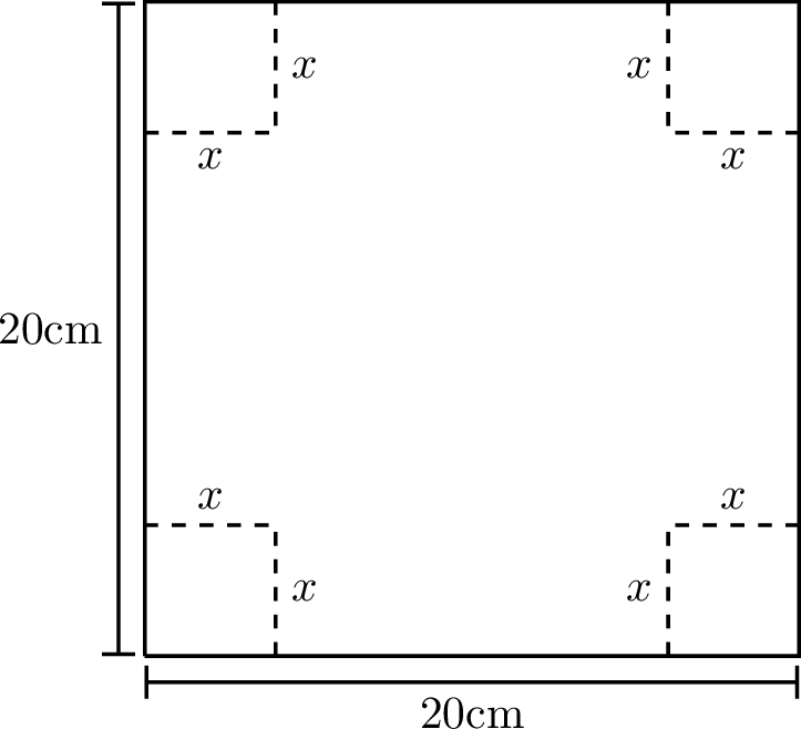
Figure 3.8: Folds to make a cardboard box
The hard part of the single variable optimization process is often solving the equation \(f'(x) = 0\). We could use numerical root finding schemes to solve this equation, but we could also potentially do better without actually finding the derivative. In the following we propose a few numerical techniques that can approximate the solution to these types of problems. The basic ideas are simple!
The intuition of numerical optimization schemes is typically to visualize the function that you’re trying to minimize or maximize and think about either climbing the hill to the top (maximization) or descending the hill to the bottom (minimization).
Some of the most common algorithms are listed below. Read through them and see which one(s) you ended up recreating? The intuition for these algorithms is pretty darn simple – travel uphill if you want to maximize – travel downhill if you want to minimize.
Definition 3.5 (Derivative Free Optimization) Let \(f(x)\) be the objective function which you are seeking to maximize (or minimize).
Pick a starting point, \(x_0\), and find the value of your objective function at this point, \(f(x_0)\).
Pick a small step size (say, \(\Delta x \approx 0.01\)).
Calculate the objective function one step to the left and one step to the right from your starting point. Which ever point is larger (if you’re seeking a maximum) is the point that you keep for your next step.
Iterate (decide on a good stopping rule)
Definition 3.6 (Gradient Descent/Ascent) Let \(f(x)\) be the objective function which you are seeking to maximize (or minimize).
Find the derivative of your objective function, \(f'(x)\).
Pick a starting point, \(x_0\).
Pick a small control parameter, \(\alpha\) (in machine learning this parameter is called the “learning rate” for the gradient descent algorithm).
Use the iteration \(x_{n+1} = x_n + \alpha f'(x_n)\) if you’re maximizing. Use the iteration \(x_{n+1} = x_n - \alpha f'(x_n)\) if you’re minimizing.
Iterate (decide on a good stopping rule)
Definition 3.7 (Monte-Carlo Search) Let \(f(x)\) be the objective function which you are seeking to maximize (or minimize).
Pick many (perhaps several thousand!) different \(x\) values.
Find the value of the objective function at every one of these points (Hint: use lists, not loops)
Keep the \(x\) value that has the largest (or smallest if you’re minimizing) value of the objective function.
Iterate many times and compare the function value in each iteration to the previous best function value
Definition 3.8 (Optimization via Numerical Root Finding) Let \(f(x)\) be the objective function which you are seeking to maximize (or minimize).
Find the derivative of your objective function.
Set the derivative to zero and use a numerical root finding method (such as bisection or Newton) to find the critical point.
Use the extreme value theorem to determine if the critical point or one of the endpoints is the maximum (or minimum).
Exercise 3.56 In this problem we will compare an contrast the four methods proposed in the previous problem.
What are the advantages to each of the methods proposed?
What are the disadvantages to each of the methods proposed?
Which method, do you suppose, will be faster in general? Why?
Which method, do you suppose, will be slower in general? Why?
A pig weighs 200 pounds and gains weight at a rate proportional to its current weight. Today the growth rate if 5 pounds per day. The pig costs 45 cents per day to keep due mostly to the price of food. The market price for pigs if 65 cents per pound but is falling at a rate of 1 cent per day. When should the pig be sold and how much profit do you make on the pig when you sell it? Write this situation as a single variable mathematical model and solve the problem analytically (by hand). Then solve the problem with all four methods outlined thus far in this section.
Reconsider the pig problem 3.58 but now suppose that the weight of the pig after \(t\) days is \[w = \frac{800}{1+3e^{-t/30}} \text{ pounds}.\] When should the pig be sold and how much profit do you make on the pig when you sell it? Write this situation as a single variable mathematical model. You should notice that the algebra and calculus for solving this problem is no longer really a desirable way to go. Use an appropriate numerical technique to solve this problem.
Exercise 3.60 Numerical optimization is often seen as quite challenging since the algorithms that we have introduced here could all get “stuck” at local extrema. To illustrate this see the function shown in Figure 3.9. How will derivative free optimization methods have trouble finding the red point starting at the black point with this function? How will gradient descent/ascent methods have trouble? Why?
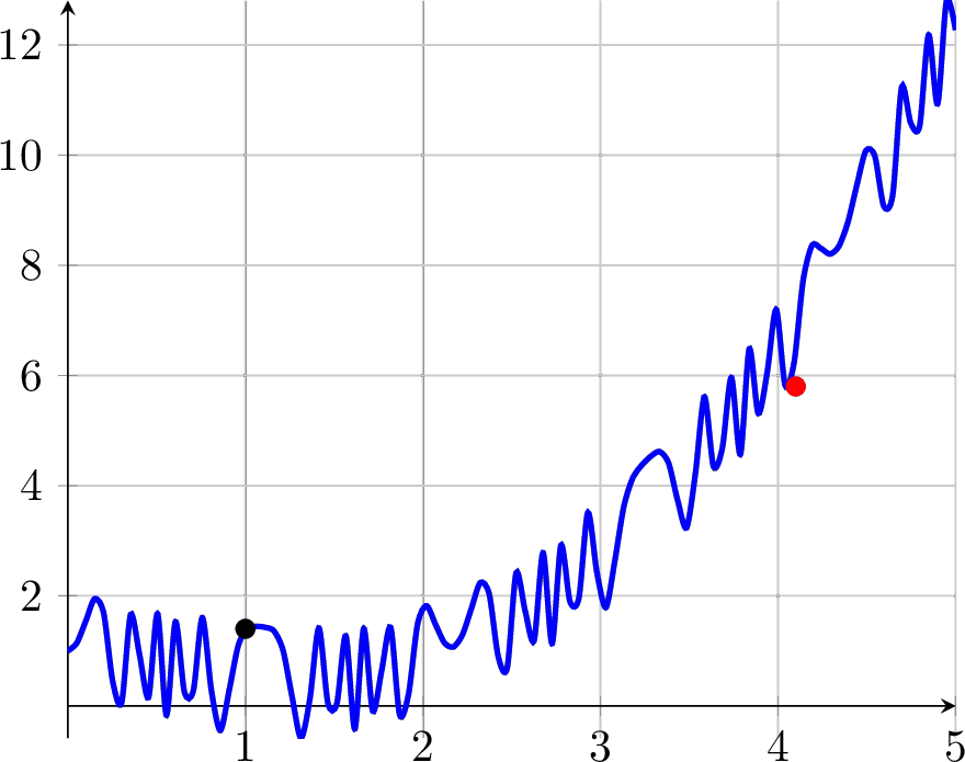
Figure 3.9: A challenging numerical optimization problem. If we start at the black point then how will any of our algorithms find the local minimum at the red point?
3.4.2 Multivariable Optimization
Now let’s look at multivariable optimization. The analytic process for finding optimal solutions is essentially the same as for single variable.
Write a function that models a scenario in multiple variables,
find the gradient vector (presuming that the function is differentiable),
set the gradient vector equal to the zero vector and solve for the critical point(s), and
interpret your answer in the context of the problem.
The trouble with unconstrained multivariable optimization is that finding the critical points is now equivalent to solving a system of nonlinear equations; a task that is likely impossible even with a computer algebra system.
Let’s see if you can extend your intuition from single variable to multivariable. This particular subsection is intentionally quite brief. If you want more details on multivariable optimization it would be wise to take a full course in optimization.
Exercise 3.61 The derivative free optimization method discussed in the single variable optimization section just said that you should pick two points and pick the one that takes you furthest uphill.
Why is it insufficient to choose just two points if we are dealing with a function of two variables? Hint: think about contour line.
For a function of two variables, how many points should you use to compare and determine the direction of “uphill?”
Extend your answer from part (b) to \(n\) dimensions. How many points should we compare if we are in \(n\) dimensions and need to determine which direction is “uphill?”
Back in the case of a two-variable function, you should have decided that three points was best. Explain an algorithm for moving one point at a time so that your three points eventually converge to a nearby local maximum. It may be helpful to make a surface plot or a contour plot of a well-known function just as a visual.
The code below will demonstrate how to make a contour plot.
import numpy as np
import matplotlib.pyplot as plt
xdomain = np.linspace(-4,4,100)
ydomain = np.linspace(-4,4,100)
X, Y = np.meshgrid(xdomain,ydomain)
f = lambda x, y: np.sin(x)*np.exp(-np.sqrt(x**2+y**2))
plt.contour(X,Y,f(X,Y))
plt.grid()
plt.show()The derivative free, gradient ascent/descent, and monte carlo techniques still have good analogues in higher dimensions. We just need to be a bit careful since in higher dimensions there is much more room to move. Below we’ll give the full description of the gradient ascent/descent algorithm. We don’t give the full description of the derivative free or Monte Carlo algorithms since there are many ways to implement them. The interested reader should see a course in mathematical optimization or machine learning.
Definition 3.9 (The Gradient Descent Algorithm) We want to solve the problem \[\text{minimize } f(x_1, x_2, \ldots, x_n) \text{ subject to }(x_1, x_2, \ldots, x_n) \in S.\]
Choose an arbitrary starting point \(\boldsymbol{x}_0 = (x_1,x_2,\ldots,x_n)\in S\).
We are going to define a difference equation that gives successive guesses for the optimal value: \[\boldsymbol{x}_{n+1} = \boldsymbol{x}_n - \alpha \nabla f(\boldsymbol{x}_n).\] The difference equation says to follow the negative gradient a certain distance from your present point (why are we doing this). Note that the value of \(\alpha\) is up to you so experiment with a few values (you should probably take \(\alpha \le 1\) …why?).
Repeat the iterative process in step b until two successive points are close enough to each other.
Take Note: If you are looking to maximize your objective function then in the Monte-Carlo search you should examine if \(z\) is greater than your current largest value. For gradient descent you should actually do a gradient ascent instead and follow the positive gradient instead of the negative gradient.
3.5 Calculus with numpy and scipy
In this section we will look at some highly versatile functions built into the numpy and scipy libraries in Python. These libraries allow us to lean on pre-built numerical routines for calculus and optimization and instead we can focus our energies on setting up the problems and interpreting solutions. The down side here is that we are going to treat some of the optimization routines in Python as black boxes, so part of the goal of this section is to partially unpack these black boxes so that we know what’s going on under the hood. If you haven’t done Exercise 2.65 yet you may want to do so now in order to get used to some of the syntax used by the Python scipy library.
3.5.1 Differentiation
There are two main tools built into the numpy and scipy libraries that do numerical differentiation. In numpy there is the np.diff() command. In scipy there is the scipy.misc.derivative() command.
np.diff() command does. Use these examples to give a thorough description for what np.diff() does to a Python list.
First example of np.diff():
import numpy as np
myList = np.arange(0,10)
print(myList)
print( np.diff(myList) )
Second example of np.diff():
import numpy as np
myList = np.linspace(0,1,6)
print(myList)
print( np.diff(myList) )
Third example of np.diff():
import numpy as np
x = np.linspace(0,1,6)
dx = x[1]-x[0]
y = x**2
dy = 2*x
print("function values: \n",y)
print("exact values of derivative: \n",dy)
print("values from np.diff(): \n",np.diff(y))
print("values from np.diff()/dx: \n",np.diff(y) / dx )np.diff() command produce a list that is one element shorter than the original list?
np.diff() to approximate the first derivative of \(f(x)\)? What is the order of the error in the approximation?
import numpy as np
x = np.linspace(0,1,6)
dx = x[1]-x[0]
y = x**2
print( np.diff(y,2) / dx**2 )np.diff() command to approximate the first and second derivatives of the function \(f(x) = x\sin(x) - \ln(x)\) on the domain \([1,5]\). Then create a plot that shows \(f(x)\) and the approximations of \(f'(x)\) and \(f''(x)\).
scipy.misc.derivative() command from the scipy library. This will be another way to calculate the derivative of a function. One advantage will be that you can just send in a Python function (or a lambda function) without actually computing the lists of values. Examine the following Python code and fully describe what it does.
import numpy as np
import scipy.misc
f = lambda x: x**2
x = np.linspace(1,5,5)
df = scipy.misc.derivative(f,x,dx = 1e-10)
print(df)
import numpy as np
x = np.linspace(0,1,6)
dx = x[1]-x[0]
y = x**2
dy = 2*x
print("function values: \n",y)
print("exact values of derivative: \n",dy)
print("values from np.diff(): \n",np.diff(y))
print("values from np.diff()/dx: \n",np.diff(y) / dx )One advantage to using scipy.misc.derivative() is that you get to dictate the error in the derivative computation, and that error is not tied to the list of values that you provide. In its simplest form you can provide just a single \(x\) value just like in the next block of code.
import numpy as np
import scipy.misc
f = lambda x: x**2
df = scipy.misc.derivative(f,1,dx = 1e-10) # derivative at x=1
print(df)scipy.misc.derivative(). Notice that we’ve chosen to take dx=1e-6 for each of the derivative computations. That may seem like an odd choice, but there is more going on here. Try successively smaller and smaller values for the dx parameter. What do you find? Why does it happen?
import numpy as np
import scipy.misc
import matplotlib.pyplot as plt
f = lambda x: np.sin(x)*x-np.log(x)
x = np.linspace(1,5,100) # x domain: 100 points between 1 and 5
df = scipy.misc.derivative(f,x,dx=1e-6)
df2 = scipy.misc.derivative(f,x,dx=1e-6,n=2)
plt.plot(x,f(x),'b',x,df,'r--',x,df2,'k--')
plt.legend(["f(x)","f'(x)","f''(x)"])
plt.grid()
plt.show()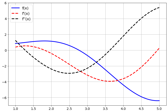
Figure 3.10: Derivatives with scipy
3.5.2 Integration
In numpy there is a nice tool called np.trapz() that implements the trapezoidal rule. In the following problem you will find several examples of the np.trapz() command. Use these examples to determine how the command works to integrate functions.
import numpy as np
x = np.linspace(-2,2,100)
dx = x[1]-x[0]
y = x**2
print("Approximate integral is ",np.trapz(y)*dx)
Next we’ll approximate \(\int_0^{2\pi} \sin(x) dx\). We know that the exact value is 0.
import numpy as np
x = np.linspace(0,2*np.pi,100)
dx = x[1]-x[0]
y = np.sin(x)
print("Approximate integral is ",np.trapz(y)*dx)
Pick a function and an interval for which you know the exact definite integral. Demonstrate how to use np.trapz() on your definite integral.
np.trapz() command by dx. Why did we do this? What is the np.trapz() command doing without the dx?
In the scipy library there is a more general tool called scipy.integrate.quad(). The term “quad” is short for “quadrature.” In numerical analysis literature rules like Simpson’s rule are called quadrature rules for integration. The function scipy.integrate.quad() accepts a Python function (or a lambda function) and the bounds of the definite integral. It outputs an approximation of the integral along with an approximation of the error in the integral calculation. See the Python code below.
import numpy as np
import scipy.integrate
f = lambda x: x**2
I = scipy.integrate.quad(f,-2,2)
print(I)scipy.integrate.quad() command as compared to the np.trapz() command.
3.5.3 Optimization
As you’ve seen in this section there are many tools built into numpy and scipy that will do some of our basic numerical computations. The same is true for numerical optimization problems. Keep in mind throughout the remainder of this section that the whole topic of numerical optimization is still an active area of research and there is much more to the story that what we’ll see here. However, the Python tools that we will use are highly optimized and tend to work quite well.
scipy.optimize.minimize() find this value for us numerically. The routine is much like Newton’s Method in that we give it a starting point near where we think the optimum will be and it will iterate through some algorithm (like a derivative free optimization routine) to approximate the minimum.
import numpy as np
from scipy.optimize import minimize
f = lambda x: (x-3)**2 - 5
minimize(f,2)- Implement the code above then spend some time playing around with the minimize command to minimize more challenging functions.
- Explain what all of the output information is from the
.minimize()command.
scipy.optimize.maximize(). Instead, Python expects you to rewrite every maximization problem as a minimization problem. How do you do that?
3.6 Least Squares Curve Fitting
In this section we’ll change our focus a bit to look at a different question from algebra, and, in turn, reveal a hidden numerical optimization problem where the scipy.optimize.minimize() tool will come in quite handy.
Here is the primary question of interest:
If we have a few data points and a reasonable guess for the type of function fitting the points, how would we determine the actual function?
You may recognize this as the basic question of regression from statistics. What we will do here is pose the statistical question of which curve best fits a data set as an optimization problem. Then we will use the tools that we’ve built so far to solve the optimization problem.
Exercise 3.80 Consider the function \(f(x)\) that goes exactly through the points \((0,1)\), \((1,4)\), and \((2,13)\).
Find a function that goes through these points exactly. Be able to defend your work.
Is your function unique? That is to say, is there another function out there that also goes exactly through these points?
Exercise 3.81 Now let’s make a minor tweak to the previous problem. Let’s say that we have the data points \((0,1.07)\), \((1,3.9)\), \((2,14.8)\), and \((3,26.8)\). Notice that these points are close to the points we had in the previous problem, but all of the \(y\) values have a little noise in them and we have added a fourth point. If we suspect that a function \(f(x)\) that best fits this data is quadratic then \(f(x) = ax^2 + bx + c\) for some constants \(a\), \(b\), and \(c\).
Plot the four points along with the function \(f(x)\) for arbitrarily chosen values of \(a\), \(b\), and \(c\).
Work with your partner(s) to systematically change \(a\), \(b\), and \(c\) so that you get a good visual match to the data. The Python code below will help you get started.
import numpy as np
import matplotlib.pyplot as plt
xdata = np.array([0, 1, 2, 3])
ydata = np.array([1.07, 3.9, 14.8, 26.8])
a = # conjecture a value of a
b = # conjecture a value of b
c = # conjecture a value of c
x = # build an x domain starting at 0 and going through 4
guess = a*x**2 + b*x + c
# make a plot of the data
# make a plot of your function on top of the data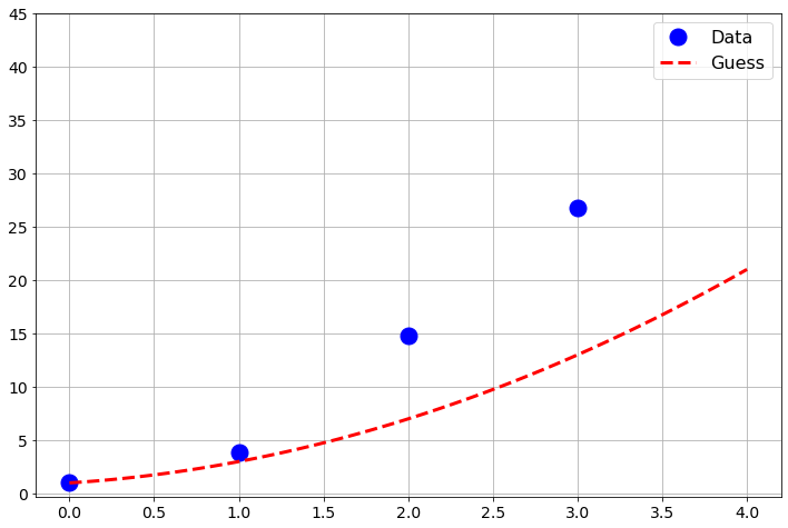
Figure 3.11: Initial attempt at matching data with a quadratic.
As an alternative to loading the data manually we could download the data from the book’s github page. All datasets in the text can be loaded in this way. We will be using the pandas library (a Python data science library) to load the .csv files.
import numpy as np
import pandas as pd
URL1 = 'https://raw.githubusercontent.com/NumericalMethodsSullivan'
URL2 = '/NumericalMethodsSullivan.github.io/master/data/'
URL = URL1+URL2
data = np.array( pd.read_csv(URL+'Exercise3_datafit1.csv') )
# Exercise3_datafit1.csv
xdata = data[:,0]
ydata = data[:,1]
Exercise 3.82 Now let’s be a bit more systematic about things from the previous problem. Let’s say that you have a pretty good guess that \(b \approx 2\) and \(c \approx 0.7\). We need to get a good estimate for \(a\).
- Pick an arbitrary starting value for \(a\) then for each of the four points find the error between the predicted \(y\) value and the actual \(y\) value. These errors are called the residuals.
- Square all four of your errors and add them up. (Pause, ponder, and discuss: why are we squaring the errors before we sum them?)
- Now change your value of \(a\) to several different values and record the sum of the square errors for each of your values of \(a\). It may be worth while to use a spreadsheet to keep track of your work here.
- Make a plot with the value of \(a\) on the horizontal axis and the value of the sum of the square errors on the vertical axis. Use your plot to defend the optimal choice for \(a\).
import numpy as np
import matplotlib.pyplot as plt
xdata = np.array([0, 1, 2, 3])
ydata = np.array([1.07, 3.9, 14.8, 26.8])
b = 2
c = 0.75
A = # give a numpy array of values for a
SumSqRes = [] # this is storage for the sum of the sq. residuals
for a in A:
  guess = a*xdata**2 + b*xdata + c
  residuals = # write code to calculate the residuals
  SumSqRes.append( ??? ) # calculate the sum of the squ. residuals
plt.plot(A,SumSqRes,'r*')
plt.grid()
plt.xlabel('Value of a')
plt.ylabel('Sum of squared residuals')
plt.show()
Now let’s formalize the process that we’ve described in the previous problems.
Definition 3.10 (Least Squares Regression) Let \[S = \{ (x_0, y_0), \, (x_1, y_1), \, \ldots, \, (x_n, y_n) \}\] be a set of \(n+1\) ordered pairs in \(\mathbb{R}^2\). If we guess that a function \(f(x)\) is a best choice to fit the data and if \(f(x)\) depends on parameters \(a_0, a_n, \ldots, a_n\) then
Pick initial values for the parameters \(a_0, a_1, \ldots, a_n\) so that the function \(f(x)\) looks like it is close to the data (this is strictly a visual step …take care that it may take some playing around to guess the initial values of the parameters)
Calculate the square error between the data point and the prediction from the function \(f(x)\) \[\text{error for the point $x_i$: } e_i = \left( y_i - f(x_i) \right)^2.\] Note that squaring the error has the advantages of removing the sign, accentuating errors larger than 1, and decreasing errors that are less than 1.
As a measure of the total error between the function and the data, sum the squared errors \[\text{sum of square errors } = \sum_{i=1}^n \left( y_i - f(x_i) \right)^2.\] (Take note that if there were a continuum of points instead of a discrete set then we would integrate the square errors instead of taking a sum.)
Change the parameters \(a_0, a_1, \ldots\) so as to minimize the sum of the square errors.
scipy.optimize.minimize() to that function in order to return the values of the parameters that best minimize the sum of the squared residuals. The following blocks of Python code implement the idea in a very streamlined way. Go through the code and comment each line to describe exactly what it does.
import numpy as np
import matplotlib.pyplot as plt
from scipy.optimize import minimize
xdata = np.array([0, 1, 2, 3])
ydata = np.array([1.07, 3.9, 14.8, 26.8])

def SSRes(parameters):
  # In the next line of code we want to build our
  # quadratic approximation y = ax^2 + bx + c
  # We are sending in a list of parameters so
  # a = parameters[0], b = parameters[1], and c = parameters[2]
  yapprox = parameters[0]*xdata**2 + \
            parameters[1]*xdata + \
            parameters[2]
  residuals = np.abs(ydata-yapprox)
  return np.sum(residuals**2)


BestParameters = minimize(SSRes,[2,2,0.75])
print("The best values of a, b, and c are: \n",BestParameters.x)
# If you want to print the diagnositc then use the line below:
# print("The minimization diagnostics are: \n",BestParameters)plt.plot(xdata,ydata,'bo',markersize=5)
x = np.linspace(0,4,100)
y = BestParameters.x[0]*x**2 + \
BestParameters.x[1]*x + \
BestParameters.x[2]
plt.plot(x,y,'r--')
plt.grid()
plt.xlabel('x')
plt.ylabel('y')
plt.title('Best Fit Quadratic')
plt.show()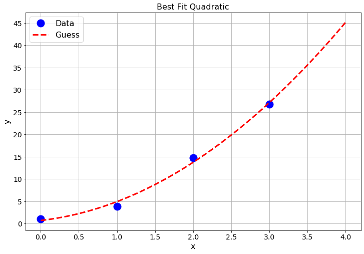
Figure 3.12: Best fit quadratic function.
Exercise 3.85 With a partner choose a function and then choose 10 points on that function. Add a small bit of error into the \(y\)-values of your points. Give your 10 points to another group. Upon receiving your new points:
- Plot your points.
- Make a guess about the basic form of the function that might best fit the data. Your general form will likely have several parameters (just like the quadratic had the parameters \(a\), \(b\), and \(c\)).
- Modify the code from above to find the best collection of parameters minimize the sum of the squares of the residuals between your function and the data.
- Plot the data along with your best fit function. If you are not satisfied with how it fit then make another guess on the type of function and repeat the process.
- Finally, go back to the group who gave you your points and check your work.
Exercise 3.86 For each dataset associated with this exercise give a functional form that might be a good model for the data. Be sure to choose the most general form of your guess. For example, if you choose “quadratic” then your functional guess is \(f(x) = ax^2 + bx + c\), if you choose “exponential” then your functional guess should be something like \(f(x) = ae^{b(x-c)}+d\), or if you choose “sinusoidal” then your guess should be something like \(f(x) = a\sin(bx) + c\cos(dx) + e\). Once you have a guess of the function type create a plot showing your data along with your guess for a reasonable set of parameters. Then write a function that leverages scipy.optimize.minimize() to find the best set of parameters so that your function best fits the data. Note that if scipy.optimize.minimize() does not converge then try the alternative scipy function scipy.optimize.fmin(). Also note that you likely need to be very close to the optimal parameters to get the optimizer to work properly.
import numpy as np
import pandas as pd
URL1 = 'https://raw.githubusercontent.com/NumericalMethodsSullivan'
URL2 = '/NumericalMethodsSullivan.github.io/master/data/'
URL = URL1+URL2
datasetA = np.array( pd.read_csv(URL+'Exercise3_datafit2.csv') )
datasetB = np.array( pd.read_csv(URL+'Exercise3_datafit3.csv') )
datasetC = np.array( pd.read_csv(URL+'Exercise3_datafit4.csv') )
# Exercise3_datafit1.csv,
# Exercise3_datafit2.csv,
# Exercise3_datafit3.csv
As a nudge in the right direction, in the left-hand pane of Figure 3.13 the function appears to be exponential. Hence we should choose a function of the form \(f(x) = ae^{b(x-c)}+d\). Moreover, we need to pick good approximations of the parameters to start the optimization process. In the left-hand pane of Figure 3.13 the data appears to start near \(x=1970\) so our initial guess for \(c\) might be \(c \approx 1970\). To get initial guesses for \(a\), \(b\), and \(d\) we can observe that the expected best fit curve will approximately go through the points \((1970,15000)\), \((1990,40000)\), and \((2000,75000)\). With this information we get the equations \(a+d \approx 15000\), \(ae^{20b}+d \approx 40000\) and \(ae^{30b}+d \approx 75000\) and work to get reasonable approximations for \(a,b,\) and \(d\) to feed into the scipy.optimize.minimize() command.
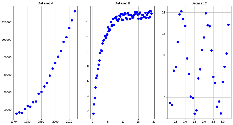
Figure 3.13: Raw data for least squares function matching problems.
3.7 Exercises
3.7.1 Algorithm Summaries
3.7.2 Applying What You’ve Learned
Exercise 3.97 For each of the following numerical differentiation formulas (1) prove
that the formula is true and (2) find the order of the method. To prove
that each of the formulas is true you will need to write the Taylor
series for all of the terms in the numerator on the right and then
simplify to solve for the necessary derivative. The highest power of the
remainder should reveal the order of the method. Simplifying hint: You may want to leverage Python’s sympy library to do some of the algebra for you.
\(f'(x) \approx \frac{\frac{1}{12} f(x-2h) - \frac{2}{3} f(x-h) + \frac{2}{3} f(x+h) - \frac{1}{12} f(x+2h)}{h}\)
\(f'(x) \approx \frac{-\frac{3}{2} f(x) + 2 f(x+h) - \frac{1}{2} f(x+2h)}{h}\)
\(f''(x) \approx \frac{-\frac{1}{12} f(x-2h) + \frac{4}{3} f(x-h) - \frac{5}{2} f(x) + \frac{4}{3} f(x+h) - \frac{1}{12} f(x+2h)}{h^2}\)
\(f'''(x) \approx \frac{-\frac{1}{2} f(x-2h) + f(x-h) - f(x+h) + \frac{1}{2} f(x+2h)}{h^3}\)
*.csv file and returns a list of \((x,y)\) ordered pairs for a
second order approximation of the second derivative of the underlying
function. Create a test spreadsheet file and a test script that have graphical
output showing that your function is finding the correct derivative.
Exercise 3.101 Use numerical integration to answer the question in each of the following scenarios
- We measure the rate at which water is flowing out of a reservoir (in gallons per second) several times over the course of one hour. Estimate the total amount of water which left the reservoir during that hour.
| time (min) | 0 | 7 | 19 | 25 | 38 | 47 | 55 |
|---|---|---|---|---|---|---|---|
| flow rate (gal/sec) | 316 | 309 | 296 | 298 | 305 | 314 | 322 |
import numpy as np
import pandas as pd
URL1 = 'https://raw.githubusercontent.com/NumericalMethodsSullivan'
URL2 = '/NumericalMethodsSullivan.github.io/master/data/'
URL = URL1+URL2
data = np.array( pd.read_csv(URL+'Exercise3_waterflow.csv') )
# Exercise3_waterflow.csv- The department of transportation finds that the rate at which cars cross a bridge can be approximated by the function \[f(t) = \frac{22.8 }{3.5 + 7(t-1.25)^4} ,\] where \(t=0\) at 4pm, and is measured in hours, and \(f(t)\) is measured in cars per minute. Estimate the total number of cars that cross the bridge between 4 and 6pm. Make sure that your estimate has an error less than 5% and provide sufficient mathematical evidence of your error estimate.
scipy.integrate.quad command. (What we’re really doing here is comparing our algorithms to Python’s scipy.integrate.quad() algorithm).
Exercise 3.103 Go to data.gov or the World Health Organization Data Repository and find data sets for the following tasks.
Find a data set where the variables naturally lead to a meaningful derivative. Use appropriate code to evaluate and plot the derivative. If your data appears to be subject to significant noise then you may want to smooth the data first before doing the derivative. Write a few sentences explaning what the derivative means in the context of the data.
Find a data set where the variables naturally lead to a meaningfun definite integral. Use appropriate code to evaluate the definite integral. If your data appears to be subject to significant noise then you might want to smooth the data first before doing the integral. Write a few sentences explaning what the integral means in the context of the data.
In both of these tasks be very cautious of the units on the data sets and the units of your answer.
Exercise 3.104 Numerically integrate each of the functions over the interval \([-1,2]\) with an appropriate technique and verify mathematically that your numerical integral is correct to 10 decimal places. Then provide a plot of the function along with its numerical first derivative.
\(f(x) = \frac{x}{1+x^4}\)
\(g(x) = (x-1)^3 (x-2)^2\)
\(h(x) = \sin\left(x^2\right)\)
Exercise 3.105 A bicyclist completes a race course in 90 seconds. The speed of the biker at each 10-second interval is determined using a radar gun and is given in the table in feet per second. How long is the race course?
| Time (sec) | 0 | 10 | 20 | 30 | 40 | 50 | 60 | 70 | 80 | 90 |
|---|---|---|---|---|---|---|---|---|---|---|
| Speed (ft/sec) | 34 | 32 | 29 | 33 | 37 | 40 | 41 | 36 | 38 | 39 |
import numpy as np
import pandas as pd
URL1 = 'https://raw.githubusercontent.com/NumericalMethodsSullivan'
URL2 = '/NumericalMethodsSullivan.github.io/master/data/'
URL = URL1+URL2
data = np.array( pd.read_csv(URL+'Exercise3_bikespeed.csv') )
# Exercise3_bikespeed.csv
Exercise 3.106 For each of the following functions write code to numerically approximate the local maximum or minimum that is closest to \(x=0\). You may want to start with a plot of the function just to get a feel for where the local extreme value(s) might be.
\(\displaystyle f(x) = \frac{x}{1+x^4} + \sin(x)\)
\(\displaystyle g(x) = \left(x-1\right)^3\cdot\left(x-2\right)^2+e^{-0.5\cdot x}\)
Exercise 3.108 In the code below you can download several sets of noisy data from measurements of elementary single variable functions.
Make a hypothesis about which type of function would best model the data. Be sure to choose the most general (parameterized) form of your function.
Use appropriate tools to find the parameters for the function that best fits the data. Report you sum of square residuals for each function.
The functions that you propose must be continuous functions.
import numpy as np
import pandas as pd
URL1 = 'https://raw.githubusercontent.com/NumericalMethodsSullivan'
URL2 = '/NumericalMethodsSullivan.github.io/master/data/'
URL = URL1+URL2
datasetA = np.array( pd.read_csv(URL+'Exercise3_datafit5.csv') )
datasetB = np.array( pd.read_csv(URL+'Exercise3_datafit6.csv') )
datasetC = np.array( pd.read_csv(URL+'Exercise3_datafit7.csv') )
datasetD = np.array( pd.read_csv(URL+'Exercise3_datafit8.csv') )
datasetE = np.array( pd.read_csv(URL+'Exercise3_datafit9.csv') )
datasetF = np.array( pd.read_csv(URL+'Exercise3_datafit10.csv') )
datasetG = np.array( pd.read_csv(URL+'Exercise3_datafit11.csv') )
datasetH = np.array( pd.read_csv(URL+'Exercise3_datafit12.csv') )
# Exercise3_datafit5.csv - Exercise3_datafit12.csv
Exercise 3.109 (The Goat Problem) This is a classic problem in recreational mathematics that has a great approximate solution where we can leverage some of our numerical analysis skills. Grab a pencil and a piece of paper so we can draw a picture.
- Draw a coordinate plane
- Draw a circle with radius 1 unit centered at the point \((0,1)\). This circle will obviously be tangent to the \(x\) axis.
- Draw a circle with radius \(r\) centered at the point \((0,0)\). We will take \(0 < r < 2\) so there are two intersections of the two circles.
- Label the left-hand intersection of the two circles as point \(A\). (Point \(A\) should be in the second quadrant of your coordinate plane.)
- Label the right-hand intersection of the circles as point \(B\). (Point \(B\) should be in the first quadrant of your coordinate plane.)
- Label the point \((0,0)\) as the point \(P\).
A rancher has built a circular fence of radius 1 unit centered at the point \((0,1)\) for his goat to graze. He tethers his goat at point \(P\) on the far south end of the circular fence. He wants to make the length of the goat’s chain, \(r\), just long enough so that it can graze half of the area of the fenced region. How long should he make the chain?
Hints:
It would be helpful to write equations for both circles. Then you can use the equations to find the coordinates of the intersection points \(A\) and \(B\).
- You can either solve for the intersection points algebraically or you can use a numerical root finding technique to find the intersection points.
- In any case, the intersection points will (obviously) depend on the value of \(r\)
Set up an integral to find the area grazed by the goat.
- You will likely need to use a numerical integration technique to evaluate the integral.
Write code to narrow down on the best value of \(r\) where the integral evaluates to half the area of the fenced region.
3.8 Projects
In this section we propose several ideas for projects related to numerical Calculus. These projects are meant to be open ended, to encourage creative mathematics, to push your coding skills, and to require you to write and communicate your mathematics. Take the time to read Appendix B before you write your final solution.
3.8.1 Galaxy Integration
To analyze the light from stars and galaxies, scientists use a spectral grating (fancy prism) to split it up into the different frequencies (colors). We can then measure the intensity (brightness) of the light (in units of Watts per square meter) at each frequency (measured in Hertz), to get intensity per frequency (Watts per square meter per Hertz, W/(m\(^2\) Hz)). Light from the dense opaque surface of a star produces a smooth rainbow, which produces a continuous curve when we plot intensity versus frequency. However stars are also surrounded by thin gas which either emits or absorbs light at only a specific set of frequencies, called spectral lines. Every chemical element produces a specific set of lines (or peaks) at fixed frequencies, so by identifying the lines, we can tell what types of atoms and molecules a star is made of. If the gas is cool, then it will absorb light at these wavelengths, and if the gas is hot then it will emit light at these wavelengths. For galaxies, on the other hand, we expect mostly emission spectra: light emitted from the galaxy.
For this project we will be analyzing the galaxy “ngc 1275.” The black hole at the center of this galaxy is often referred to as the “Galactic Spaghetti Monster” since the magnetic field “sustains a mammoth network of spaghetti-like gas filaments around it.” You can download the data file associated with this project with the following Python code.
import numpy as np
import pandas as pd
URL1='https://raw.githubusercontent.com/NumericalMethodsSullivan'
URL2='/NumericalMethodsSullivan.github.io/master/data/'
URL = URL1+URL2
ngc1275 = np.array( pd.read_csv(URL+'ngc1275.csv') )
# ngc1275.csv
In the data you will see the spectral data measuring the light intensity from ncg 1275 at several different wavelengths (measured in Angstroms ). You will notice in this data set that there are several emission lines at various wavelengths. Of particular interest are the peaks near \(3800\) Angstroms, \(5100\) Angstroms, \(6400\) Angstroms, and the two peaks around \(6700\) Angstroms. The data set contains 1,727 data points at different wavelengths. Your first job will be to transform the wavelength data to frequency via the formula \[\lambda = \frac{c}{f}\] where \(\lambda\) is the wavelength, \(c\) is the speed of light, and \(f\) is the frequency (measured in Hertz). Be sure to double check the units. Given the inverse relationship between frequency and wavelength you should see the emission lines flip to the other side of the plot (right-to-left or left-to-right).
The strength of each emission line (in W/m\(^2\)) is defined as the relative intensity of each peak across the associated frequencies. Note that you are not interested in the intensity of the continuous spectrum – just the peaks. That is to say that you are only interested in the area above the background curve and the background noise.
Your primary task is to develop a process for analyzing data sets like this so as to determine the strength of each emission lines. You must demonstrate your process on this particular data set, but your process must be generalizable to any similar data set. Your process must clearly determine the strength of peaks in data sets like this and you must apply your procedure to determine the strength of each of these four lines with an associated margin of error. Keep in mind that you will first want to first develop a method for removing the background noise. Finally, the double peak near \(6700\) Angstroms needs to be handled with care: the strength of each emission line is only the integral over one peak, not two, so you’ll need to determine a way to separate these peaks.
Finally, it would be cool, but is not necessary, to report on which chemicals correspond to the emission lines in the data. Remember that the galaxy is far away and hence there is a non-trivial red-shift to consider. This will take some research but if done properly will likely give a lot more merit to your paper.
3.8.2 Higher Order Integration
Riemann sums can be used to approximate integrals and they do so by using piecewise constant functions to approximate the function. The trapezoidal rule uses piece wise linear functions to approximate the function and then the area of a trapezoid to approximate the area. We saw earlier that Simpson’s rule uses piece wise parabolas to approximate the function. The process which we used to build Simpson’s rule can be extended to any higher-order polynomial. Your job in this project is to build integration algorithms that use piece wise cubic functions, quartic functions, etc. For each you need to show all of the mathematics necessary to derive the algorithm, provide several test cases to show that the algorithm works, and produce a numerical experiment that shows the order of accuracy of the algorithm.
3.8.3 Dam Integration
Go to the USGS water data repository:
https://maps.waterdata.usgs.gov/mapper/index.html.
Here you’ll find a map with information about water resources around the
country.
Zoom in to a dam of your choice (make sure that it is a dam).
Click on the map tag then click “Access Data”
From the drop down menu at the top select either “Daily Data” or “Current / Historical Data.” If these options don’t appear then choose a different dam.
Change the dates so you have the past year’s worth of information.
Select “Tab-separated” under “Output format” and press Go. Be sure that the data you got has a flow rate (ft\(^3\)/sec).
At this point you should have access to the entire data set. Copy it into a
csvfile and save it to your computer.
For the data that you just downloaded you have three tasks: (1) plot the data in a reasonable way giving appropriate units, (2) find the total amount of water that has been discharged from the dam during the past calendar year, and (3) report any margin of error in your calculation based on the numerical method that you used in part (2).
3.8.4 Edge Detection in Images
Edge detection is the process of finding the boundaries or edges of objects in an image. There are many approaches to performing edge detection, but one method that is quite robust is to use the gradient vector in the following way:
- First convert the image to gray scale.
- Then think of the gray scale image as a plot of a multivariable function \(G(x,y)\) where the ordered pair \((x,y)\) is the pixel location and the output \(G(x,y)\) is the value of the gray scale at that point.
- At each pixel calculate the gradient of the function \(G(x,y)\) numerically.
- If the magnitude of the gradient is larger than some threshold then the function \(G(x,y)\) is steep at that location and it is possible that there is an edge (a transition from one part of the image to a different part) at that point. Hence, if \(\|\nabla G(x,y)\| > \delta\) for some threshold \(\delta\) then we can mark the point \((x,y)\) as an edge point.
Your Tasks:
- Choose several images on which to do edge detection. You should take your own images, but if you choose not to be sure that you cite the source(s) of your images.
- Write Python code that performs edge detection as described above on the image. In the end you should produce side-by-side plots of the original picture and the image showing only the edges. To calculate the gradient use a centered difference scheme for the first derivatives
\[ f'(x) \approx \frac{f(x+h)-f(x-h)}{2h}. \]
In an image we can take \(h=1\) (why?), and since the gradient is two dimensional we get
\[ \nabla G(x,y) \approx \left< \frac{G(x+1,y)-G(x-1,y)}{2} \, , \, \frac{G(x,y+1)-G(x,y-1)}{2} \right>. \]
Figure 3.14 depicts what this looks like when we zoom in to a pixel and its immediate neighbors. The pixel labeled
G[i,j]is the pixel at which we want to evaluate the gradient, and the surrounding pixels are labeled by their indices relative to[i,j].
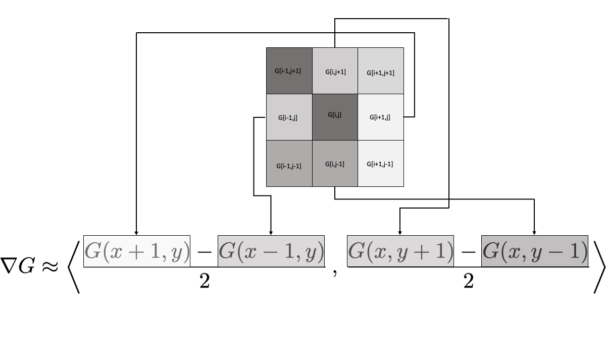
Figure 3.14: The gradient computation on a single pixel using a centered difference scheme for the first derivative.
- There are many ways to approximate numerical first derivatives. The simplest approach is what you did in part (2) – using a centered difference scheme. However, pixels are necessarily tightly packed in an image and the immediate neighbors of a point may not have enough contrast to truly detect edges. If you examine Figure 3.14 you’ll notice that we only use 4 of the 8 neighbors of the pixel
[i,j]. Also notice that we didn’t reach out any further than a single pixel. Your job now is to build several other approaches to calculating the gradient vector, implement them to perform edge detection, and show the resulting images. For each method you need to give the full mathematical details for how you calculated the gradient as well as give a list of pros and cons for using the new numerical gradient for edge detection based on what you see in your images. As an example, you could use a centered difference scheme that looks two pixels away instead of at the immediate neighboring pixels \[ f'(x) \approx \frac{??? f(x-2) + ??? f(x+2)}{???}. \] Of course you would need to determine the coefficients in this approximation scheme.
Another idea could use a centered difference scheme that uses pixels that are immediate neighbors AND pixels that are two units away \[ f'(x) \approx \frac{??? f(x-2) + ??? f(x-1) + ??? f(x+1) + ??? f(x+2)}{???}. \]
In any case, you will need to use Taylor Series to derive coefficients in the formulas for the derivatives as well as the order of the error. There are many ways to approximate the first derivatives so be creative. In your exploration you are not restricted to using just the first derivative. There could be some argument for using the second derivatives and/or the Hessian matrix of the gray scale image function \(G(x,y)\) and using some function of the concavity as a means of edge detection. Explore and have fun!
The following code will allow you to read an image into Python as an np.array().
import numpy as np
import matplotlib.pyplot as plt
from matplotlib import image
I = np.array(image.plt.imread('ImageName.jpg'))
plt.imshow(I)
plt.axis("off")
plt.show()
You should notice that the image, I, is a three dimensional array. The three layers are the red, green, and blue channels of the image. To flatten the image to gray scale you can apply the rule
\[ \text{grayscale value} = 0.3 \text{Red} + 0.59 \text{Green} + 0.11 \text{Blue}. \]
The output should be a 2 dimensional numpy array which you can show with the following Python code.
plt.imshow(G, cmap='gray') # "cmap" stands for "color map"
plt.axis("off")
plt.show()
Figure 3.15 shows the result of different threshold values applied to the simplest numerical gradient computations. The image was taken by the author.
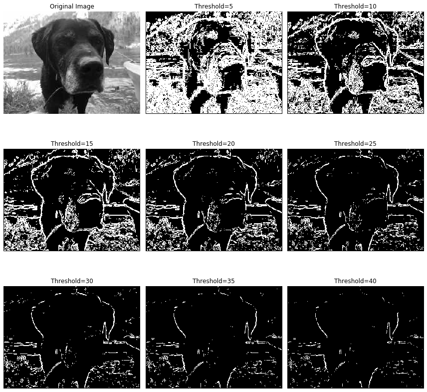
Figure 3.15: Edge detection using different thresholds for the value of the gradient on the grayscale image