1 Preliminary Topics

1.1 What Is Numerical Analysis?

“In the 1950s and 1960s, the founding fathers of Numerical Analysis discovered that inexact arithmetic can be a source of danger, causing errors in results that ‘ought’ to be right. The source of such problems is numerical instability: that is, the amplification of rounding errors from microscopic to macroscopic scale by certain modes of computation.”
–Oxford Professor Lloyd (Nick) Trefethen (2006)

The field of Numerical Analysis is really the study of how to take mathematical problems and perform them efficiently and accurately on a computer. While the field of numerical analysis is quite powerful and wide-reaching, there are some mathematical problems where numerical analysis doesn’t make much sense (e.g. finding an algebraic derivative of a function, proving a theorem, uncovering a pattern in a sequence). However, for many problems a numerical method that gives an approximate answer is both more efficient and more versatile than any analytic technique. Let’s look at several examples. You can also watch a short introduction video here: https://youtu.be/yH0zhca0hbs

Example from Algebra:: Solve the equation $\ln(x) = \sin(x)$ for $x$ in the interval $x \in (0,\pi)$. Stop and think about all of the algebra that you ever learned. You’ll quickly realize that there are no by-hand techniques that can solve this problem! A numerical approximation, however, is not so hard to come by.
Example from Calculus:: What if we want to evaluate the following integral? \[ \int_0^\pi \sin(x^2) dx \] Again, trying to use any of the possible techniques for using the Fundamental Theorem of Calculus, and hence finding an antiderivative, on the function $\sin(x^2)$ is completely hopeless. Substitution, integration by parts, and all of the other techniques that you know will all fail. Again, a numerical approximation is not so difficult and is very fast! By the way, this integral (called the Fresnel Sine Integral) actually shows up naturally in the field of optics and electromagnetism, so it is not just some arbitrary integral that I cooked up just for fun.
Example from Differential Equations:: Say we needed to solve the differential equation $\frac{dy}{dt} = \sin(y^2) + t.$ The nonlinear nature of the problem precludes us from using most of the typical techniques (e.g. separation of variables, undetermined coefficients, Laplace Transforms, etc). However, computational methods that result in a plot of an approximate solution can be made very quickly and likely give enough of a solution to be usable.
Example from Linear Algebra:: You have probably never row reduced a matrix larger than $3\times 3$ or perhaps $4 \times 4$ by hand. Instead, you often turn to technology to do the row reduction for you. You would be surprised to find that the standard row reduction algorithm (RREF) that you do by hand is not what a computer uses. Instead, there are efficient algorithms to do the basic operations of linear algebra (e.g. Gaussian elimination, matrix factorization, or eigenvalue decomposition)

In this chapter we will discuss some of the basic underlying ideas in Numerical Analysis, and the essence of the above quote from Nick Trefethen will be part of the focus of this chapter. Particularly, we need to know how a computer stores numbers and when that storage can get us into trouble. On a more mathematical side, we offer a brief review of the Taylor Series from Calculus at the end of this chapter. The Taylor Series underpins many of our approximation methods in this class. Finally, at the end of this chapter we provide several coding exercises that will help you to develop your programming skills. It is expected that you know some of the basics of programming before beginning this class. If you need to review the basics then see Appendix A

You’ll have more than just the basics by the end.

Let’s begin.

1.2 Arithmetic in Base 2

Exercise 1.1 By hand (no computers!) compute the first 50 terms of this sequence with the initial condition $x_0 = 1/10$. \[x_{n+1} = \left\{ \begin{array}{ll} 2x_n, & x_n \in [0,\frac{1}{2}] \\ 2x_n - 1, & x_n \in (\frac{1}{2},1] \end{array} \right.\]

Exercise 1.2 Now use a spreadhseet and to do the computations. Do you get the same answers?

Exercise 1.3 Finally, solve this problem with Python. Some starter code is given to you below.

x = 1.0/10
for n in range(50):
    if x<= 0.5:
        # put the correct assignment here
    else:
        # put the correct assigment here
    print(x)

Exercise 1.4 It seems like the computer has failed you! What do you think happened on the computer and why did it give you a different answer? What, do you suppose, is the cautionary tale hiding behind the scenes with this problem?

Exercise 1.5 Now what happens with this problem when you start with $x_0 = 1/8$? Why does this new initial condition work better?

A computer circuit knows two states: on and off. As such, anything saved in computer memory is stored using base-2 numbers. This is called a binary number system. To fully understand a binary number system it is worth while to pause and reflect on our base-10 number system for a few moments.

What do the digits in the number “$735$” really mean? The position of each digit tells us something particular about the magnitude of the overall number. The number $735$ can be represented as a sum of powers of $10$ as \[735 = 700 + 30 + 5 = 7 \times 10^2 + 3 \times 10^1 + 5 \times 10^0\] and we can read this number as $7$ hundreds, $3$ tens, and $5$ ones. As you can see, in a “positional number system” such as our base-10 system, the position of the number indicates the power of the base, and the value of the digit itself tells you the multiplier of that power. This is contrary to number systems like Roman Numerals where the symbols themselves give us the number, and meaning of the position is somewhat flexible. The number “48,329” can therefore be interpreted as \[48,329 = 40,000 + 8,000 + 300 + 20 + 9 = 4 \times 10^4 + 8 \times 10^3 + 3 \times 10^2 + 2 \times 10^1 + 9 \times 10^0,\] Four ten thousands, eight thousands, three hundreds, two tens, and nine ones.

Now let’s switch to the number system used by computers: the binary number system. In a binary number system the base is 2 so the only allowable digits are 0 and 1 (just like in base-10 the allowable digits were 0 through 9). In binary (base-2), the number “$101,101$” can be interpreted as \[101,101_2 = 1 \times 2^5 + 0 \times 2^4 + 1 \times 2^3 + 1 \times 2^2 + 0 \times 2^1 + 1 \times 2^0\] (where the subscript “2” indicates the base to the reader). If we put this back into base 10, so that we can read it more comfortably, we get \[101,101_2 = 32 + 0 + 8 + 4 + 0 + 1 = 45_{10}.\] The reader should take note that the commas in the numbers are only to allow for greater readability – we can easily see groups of three digits and mentally keep track of what we’re reading.

Exercise 1.6 Express the following binary numbers in base-10.

$111_2$
$10,101_2$
$1,111,111,111_2$

Exercise 1.7 Explain the joke: There are 10 types of people. Those who understand binary and those who don’t.

Exercise 1.8 Discussion: With your group discuss how you would convert a base-10 number into its binary representation. Once you have a proposed method put it into action on the number $237_{10}$ to show that the base-2 expression is $11,101,101_2$

Exercise 1.9 Convert the following numbers from base 10 to base 2 or visa versa.

Write $12_{10}$ in binary
Write $11_{10}$ in binary
Write $23_{10}$ in binary
Write $11_2$ in base 10
What is $100101_2$ in base $10$?

Exercise 1.10 Now that you have converted several base-10 numbers to base-2, summarize an efficient technique to do the conversion.

Example 1.1 Convert the number 137 from base 10 to base 2.
Solution: One way to do the conversion is to first look for the largest power of 2 less than or equal to your number. In this case, $128=2^7$ is the largest power of 2 that is less than 137. Then looking at the remainder, 9, look for the largest power of 2 that is less than this remainder. Repeat until you have the number. \[\begin{aligned} 137_{10} &= 128 + 8 + 1 \\ &= 2^7 + 2^3 + 2^0 \\ &= 1 \times 2^7 + 0 \times 2^6 + 0 \times 2^5 + 0 \times 2^4 + 1 \times 2^3 + 0 \times 2^2 + 0 \times 2^1 + 1 \times 2^0 \\ &= 10001001_2 \end{aligned}\]

Next we’ll work with fractions and decimals. For example, let’s take the base 10 number $5.341_{10}$ and expand it out to get \[5.341_{10} = 5 + \frac{3}{10} + \frac{4}{100} + \frac{1}{1000} = 5 \times 10^0 + 3 \times 10^{-1} + 4 \times 10^{-2} + 1 \times 10^{-3}.\] The position to the right of the decimal point is the negative power of 10 for the given position. We can do a similar thing with binary decimals.

Exercise 1.11 The base-2 number $1,101.01_2$ can be expanded in powers of 2. Fill in the question marks below and observe the pattern in the powers. \[1,101.01_2 = ? \times 2^3 + 1 \times 2^2 + 0 \times 2^1 + ? \times 2^0 + 0 \times 2^{?} + 1 \times 2^{-2}.\]

Exercise 1.12 Repeating digits in binary numbers are rather intriguing. The number $0.\overline{0111} = 0.01110111011101110111\ldots$ surely also has a decimal representation. I’ll get you started: \[\begin{aligned} 0.0_2 &= 0 \times 2^0 + 0 \times 2^{-1} = 0.0_{10} \\ 0.01_2 &= 0.0_{10} + 1 \times 2^{-2} = 0.25_{10} \\ 0.011_2 &= 0.25_{10} + 1 \times 2^{-3} = 0.25_{10} + 0.125_{10} = 0.375_{10} \\ 0.0111_2 &= 0.375_{10} + 1 \times 2^{-4} = 0.4375_{10} \\ 0.01110_2 &= 0.4375_{10} + 0 \times 2^{-5} = 0.4375_{10} \\ 0.011101_2 &= 0.4375_{10} + 1 \times 2^{-6} = 0.453125_{10} \\ \vdots & \qquad \qquad \vdots \qquad \qquad \qquad \vdots \end{aligned}\] We want to know what this series converges to in base 10. Work with your partners to approximate the base-10 number.

Example 1.2 Convert $11.01011_2$ to base 10.
Solution: \[\begin{aligned} 11.01011_2 &= 2 + 1 + \frac{0}{2} + \frac{1}{4} + \frac{0}{8} + \frac{1}{16} + \frac{1}{32} \\ &= 1 \times 2^1 + 1 \times 2^0 + 0 \times 2^{-1} + 1 \times 2^{-2} + 0 \times 2^{-3} + 1 \times 2^{-4} + 1 \times 2^{-5}\\ &= 3.34375_{10}. \end{aligned}\]

Exercise 1.13 Convert the following numbers from base 10 to binary.

What is $1/2$ in binary?
What is $1/8$ in binary?
What is $4.125$ in binary?
What is $0.15625$ in binary?

Exercise 1.14 Convert the base 10 decimal $0.635$ to binary using the following steps.

Multiply $0.635$ by 2. The whole number part of the result is the first binary digit to the right of the decimal point.
Take the result of the previous multiplication and ignore the digit to the left of the decimal point. Multiply the remaining decimal by 2. The whole number part is the second binary decimal digit.
Repeat the previous step until you have nothing left, until a repeating pattern has revealed itself, or until your precision is close enough.

Explain why each step gives the binary digit that it does.

Exercise 1.15 Based on your previous problem write an algorithm that will convert base-10 decimals (less than 1) to base decimal expansions.

Exercise 1.16 Convert the base 10 fraction $1/10$ into binary. Use your solution to fully describe what went wrong in the Exercise 1.1.

1.3 Floating Point Arithmetic

Everything stored in the memory of a computer is a number, but how does a computer actually store a number. More specifically, since computers only have finite memory we would really like to know the full range of numbers that are possible to store in a computer. Moreover, since there is finite space in a computer we can only ever store rational numbers (stop and think: why is this). Therefore we need to know what gaps in our number system to expect when using a computer to store and do computations on numbers.

Exercise 1.17 Let’s start the discussion with a very concrete example. Consider the number $x = -123.15625$ (in base 10). As we’ve seen this number can be converted into binary. Indeed \[x = -123.15625_{10} = -1111011.00101_2\] (you should check this).

If a computer needs to store this number then first they put in the binary version of scientific notation. In this case we write \[x = -1. \underline{\hspace{1in}} \times 2^{\underline{\hspace{0.25in}}}\]
Based on the fact that every binary number, other than 0, can be written in this way, what three things do you suppose a computer needs to store for any given number?
Using your answer to part (b), what would a computer need to store for the binary number $x=10001001.1100110011_2$?

For any base-2 number $x$ we can write \[x = (-1)^{s} \times (1+ m) \times 2^E\] where $s \in \{0,1\}$ is called the sign bit and $m$ is a binary number such that $0 \le m < 1$.

For a number $x = (-1)^{s} \times (1+m) \times 2^E$ stored in a computer, the number $m$ is called the mantissa or the significand, $s$ is known as the sign bit, and $E$ is known as the exponent.

Example 1.3 What are the mantissa, sign bit, and exponent for the numbers $7_{10}$, $-7_{10}$, and $(0.1)_{10}$?
Solution:

For the number $7_{10}=111_2 = 1.11 \times 2^2$ we have $s=0$, $m=0.11$ and $E=2$.
For the number $-7_{10}=111_2 = -1.11 \times 2^2$ we have $s=1$, $m=0.11$ and $E=2$.
For the number $\frac{1}{10} = 0.000110011001100\cdots = 1.100110011 \times 2^{-4}$ we have $s=0$, $m=0.100110011\cdots$, and $E = -4$.

In the last part of the previous example we saw that the number $(0.1)_{10}$ is actually a repeating decimal in base-2. This means that in order to completely represent the number $(0.1)_{10}$ in base-2 we need infinitely many decimal places. Obviously that can’t happen since we are dealing with computers with finite memory. Over the course of the past several decades there have been many systems developed to properly store numbers. The IEEE standard that we now use is the accumulated effort of many computer scientists, much trial and error, and deep scientific research. We now have three standard precisions for storing numbers on a computer: single, double, and extended precision. The double precision standard is what most of our modern computers use.

Definition 1.1 There are three standard precisions for storing numbers in a computer.

A single-precision number consists of 32 bits, with 1 bit for the sign, 8 for the exponent, and 23 for the significand.
A double-precision number consists of 64 bits with 1 bit for the sign, 11 for the exponent, and 52 for the significand.
An extended-precision number consists of 80 bits, with 1 bit for the sign, 15 for the exponent, and 64 for the significand.

Definition 1.2 (machine precision) Machine precision is the gap between the number 1 and the next larger floating point number. Often it is represented by the symbol $\epsilon$. To clarify, the number 1 can always be stored in a computer system exactly and if $\epsilon$ is machine precision for that computer then $1+\epsilon$ is the next largest number that can be stored with that machine.

For all practical purposes the computer cannot tell the difference between two numbers if the difference is smaller than machine precision. This is of the utmost important when you want to check that something is “zero” since a computer just cannot know the difference between $0$ and $\epsilon$.

Exercise 1.18 To make all of these ideas concrete let’s play with a small computer system where each number is stored in the following format: \[ s \, E \, b_1 \, b_2 \, b_3 \]

The first entry is a bit for the sign (0$=+$ and $1=-$). The second entry, $E$ is for the exponent, and we’ll assume in this example that the exponent can be 0, 1, or $-1$. The three bits on the right represent the significand of the number. Hence, every number in this number system takes the form \[(-1)^s \times (1+ 0.b_1b_2b_3) \times 2^{E}\]

What is the smallest positive number that can be represented in this form?
What is the largest positive number that can be represented in this form?
What is the machine precision in this number system?
What would change if we allowed $E \in \{-2,-1,0,1,2\}$?

Exercise 1.19 What are the largest and smallest numbers that can be stored in single and double precision?

Exercise 1.20 What is machine precision for the single and double precision standard?

Exercise 1.21 Explain the behavior of the sequence from the first problem in these notes using what you know about how computers store numbers in double precision. \[x_{n+1} = \left\{ \begin{array}{ll} 2x_n, & x_n \in [0,\frac{1}{2}] \\ 2x_n - 1, & x_n \in (\frac{1}{2},1] \end{array} \right. \quad \text{with} \quad x_0 = \frac{1}{10}\] In particular, now that you know about how numbers are stored in a computer, how long do you expect it to take until the truncation error creeps into the computation?

Much more can be said about floating point numbers such as how we store infinity, how we store NaN, and how we store 0. The Wikipedia page for floating point arithmetic might be of interest for the curious reader. It is beyond the scope of this class and this book to go into all of those details here. Instead, the biggest takeaway points from this section and the previous are:

All numbers in a computer are stored with finite precision.
Nice numbers like 0.1 are sometimes not machine representable in binary.
Machine precision is the gap between 1 and the next largest number that can be stored.
Computers cannot tell the difference between two numbers if the difference is less than machine precision.

1.4 Approximating Functions

Numerical analysis is all about doing mathematics on a computer in accurate and predictable ways. Since a computer can only ever store finite bits of information for any number, most of what we do in a computer is naturally an approximation of the real mathematics. In this section we will look at a very powerful way to approximate mathematical functions.

How does a computer understand a function like $f(x) = e^x$ or $f(x) = \sin(x)$ or $f(x) = \ln(x)$? What happens under the hood, so to speak, when you ask a computer to do a computation with one of these functions? A computer is darn good at arithmetic, but working with transcendental functions like these, or really any other sufficiently complicated functions for that matter, causes all sorts of problems in a computer. Approximation of the function is something that is always happening under the hood.

Exercise 1.22 In this problem we’re going to make a bit of a wish list for all of the things that a computer will do when approximating a function. We’re going to complete the following sentence:
If we are going to approximate $f(x)$ near the point $x=x_0$ with a simpler function $g(x)$ then …

(I’ll get us started with the first two things that seems natural to wish for. The rest of the wish list is for you to complete.)

the functions $f(x)$ and $g(x)$ should agree at $x=x_0$. In other words, $f(x_0) = g(x_0)$
the function $g(x)$ should only involve addition, subtraction, multiplication, division, and integer exponents since computer are very good at those sorts of operations.
if $f(x)$ is increasing / decreasing to the right of $x=x_0$ then $g(x)$ …
if $f(x)$ is increasing / decreasing to the left of $x=x_0$ then $g(x)$ …
if $f(x)$ is concave up / down to the right of $x=x_0$ then $g(x)$…
if $f(x)$ is concave up / down to the left of $x=x_0$ then $g(x)$ …
if we zoom into plots of the functions $f(x)$ and $g(x)$ near $x=x_0$ then …
… is there anything else that you would add?

Exercise 1.23 Discuss: Could a polynomial function with a high enough degree satify everything in the wish list from the previous problem? Explain your reasoning.

Exercise 1.24 Let’s put some parts of the wish list into action. If $f(x)$ is a differentiable function at $x=x_0$ and if $g(x) = A + B (x-x_0) + C (x-x_0)^2 + D (x-x_0)^3$ then

What is the value of $A$ such that $f(x_0) = g(x_0)$? (Hint: substitute $x=x_0$ into the $g(x)$ function)
What is the value of $B$ such that $f'(x_0) = g'(x_0)$? (Hint: Start by taking the derivative of $g(x)$)
What is the value of $C$ such that $f''(x_0) = g''(x_0)$?
What is the value of $D$ such that $f'''(x_0) = g'''(x_0)$?

Exercise 1.25 Let $f(x) = e^x$. Put the answers to the previous question into action and build a cubic polynomial that approximates $f(x) = e^x$ near $x_0=0$.

In the previous 4 exercises you have built up some basic intuition for what we would want out of a mathematical operation that might build an approximation of a complicated function. What we’ve built is actually a way to get better and better approximations for functions out to pretty much any arbitrary accuracy that we like so long as we are near some anchor point (which we called $x_0$ in the previous exercises).

In the next several problems you’ll unpack the approximations of $f(x) = e^x$ a bit more carefully and we’ll wrap the whole discussion with a little bit of formal mathematical language. Then we’ll examine other functions like sine, cosine, logarithms, etc. One of the points of this whole discussion is to give you a little glimpse as to what is happening behind the scenes in scientific programming languages when you do computations with these functions. A bigger point is to start getting a feel for how we might go in reverse and approximate an unknown function out of much simpler parts. This last goal is one of the big takeaways from numerical analysis: we can mathematically model highly complicated functions out of fairly simple pieces.

Exercise 1.26 What is Euler’s number $e$? You likely remember using this number often in Calculus and Differential Equations. Do you know the decimal approximation for this number? Moreover, is there a way that we could approximate something like $\sqrt{e} = e^{0.5}$ or $e^{-1}$ without actually having access to the full decimal expansion?

For all of the questions below let’s work with the function $f(x) = e^x$.

The function $g(x) = 1$ matches $f(x) = e^x$ exactly at the point $x=0$ since $f(0) = e^0 = 1$. Furthermore if $x$ is very very close to $0$ then the functions $f(x)$ and $g(x)$ are really close to each other. Hence we could say that $g(x) = 1$ is an approximation of the function $f(x) = e^x$ for values of $x$ very very close to $x=0$. Admittedly, though, it is probably pretty clear that this is a horrible approximation for any $x$ just a little bit away from $x=0$.
Let’s get a better approximation. What if we insist that our approximation $g(x)$ matches $f(x) = e^x$ exactly at $x=0$ and ALSO has exactly the same first derivative as $f(x)$ at $x=0$.
1. What is the first derivative of $f(x)$?
2. What is $f'(0)$?
3. Use the point-slope form of a line to write the equation of the function $g(x)$ that goes through the point $(0,f(0))$ and has slope $f'(0)$. Recall from algebra that the point-slope form of a line is $y = f(x_0) + m(x-x_0).$ In this case we are taking $x_0 = 0$ so we are using the formula $g(x) = f(0) + f'(0) (x-0)$ to get the equation of the line.
Write Python code to build a plot like Figure 1.1. This plot shows $f(x) = e^x$, our first approximation $g(x) = 1$ and our second approximation $g(x) = 1+x$.

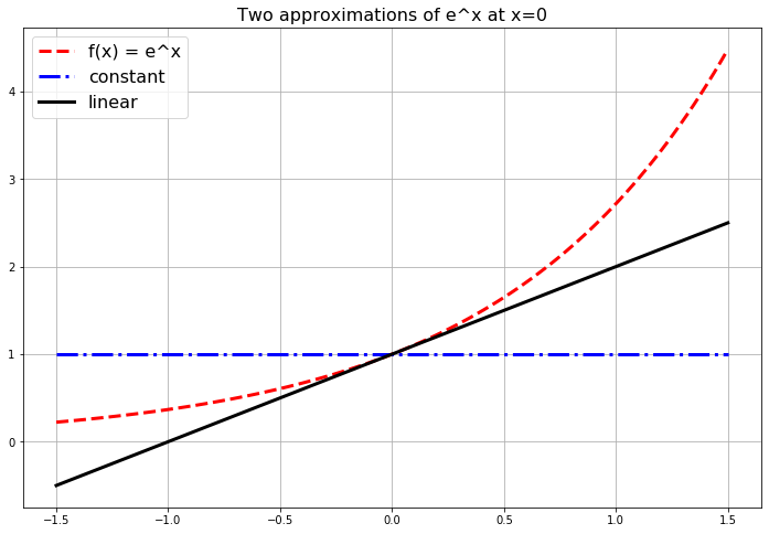
Figure 1.1: The first few polynomial approximations of the exponential function.

Exercise 1.27 Let’s extend the idea from the previous problem to much better approximations of the function $f(x) = e^x$.

Let’s build a function $g(x)$ that matches $f(x)$ exactly at $x=0$, has exactly the same first derivative as $f(x)$ at $x=0$, AND has exactly the same second derivative as $f(x)$ at $x=0$. To do this we’ll use a quadratic function. For a quadratic approximation of a function we just take a slight extension to the point-slope form of a line and use the equation \[ y = f(x_0) + f'(x_0) (x-x_0) + \frac{f''(x_0)}{2} (x-x_0)^2. \] In this case we are using $x_0 = 0$ so the quadratic approximation function looks like \[ y = f(0) + f'(0) x + \frac{f''(0)}{2} x^2. \]
1. Find the quadratic approximation for $f(x) = e^x$.
2. How do you know that this function matches $f(x)$ is all of the ways described above at $x=0$?
3. Add your new function to the plot you created in the previous problem.
Let’s keep going!! Next we’ll do a cubic approximation. A cubic approximation takes the form \[ y = f(x_0) + f'(0) (x-x_0) + \frac{f''(0)}{2}(x-x_0)^2 + \frac{f'''(0)}{3!}(x-x_0)^3 \]
1. Find the cubic approximation for $f(x) = e^x$.
2. How do we know that this function matches the first, second, and third derivatives of $f(x)$ at $x=0$?
3. Add your function to the plot.
4. Pause and think: What’s the deal with the $3!$ on the cubic term?
Your turn: Build the next several approximations of $f(x) = e^x$ at $x=0$. Add these plots to the plot that we’ve been building all along.

Exercise 1.28 We can get a decimal expansion of $e$ pretty easily: \[ e \approx 2.718281828459045 \] In Python just type np.exp(1) which will just evaluate $f(x) = e^x$ at $x=1$ (and hence giving you a value for $e^1 = e$). We built our approximations in the previous problems centered at $x=0$, and $x=1$ is not too terribly far from $x=0$ so perhaps we can get a good approximation with the functions that we’ve already built. Complete the following table to see how we did with our approximations.

Approximation Function	Value at $x=1$	Absolute Error
Constant	1	$\| 2.71828... - 1\| \approx 1.71828...$
Linear	1+1=2	$\|2.71828... - 2\| \approx 0.71828...$
Quadratic
Cubic
Quartic
Quintic

Exercise 1.29 Use the functions that you’ve built to approximate $\sqrt{e} = e^{0.5}$. Check the accuracy of your answer using np.exp(0.5) in Python.

Exercise 1.30 Use the functions that you’ve built to approximate $\frac{1}{e} = e^{-1}$. Check the accuracy of your answer using np.exp(-1) in Python.

What we’ve been exploring so far in this section is the Taylor Series of a function.

Definition 1.3 (Taylor Series)If $f(x)$ is an infinitely differentiable function at the point $x_0$ then \[ f(x) = f(x_0) + f'(x_0)(x-x_0) + \frac{f''(x_0)}{2}(x-x_0)^2 + \cdots \frac{f^{(n)}(x_0)}{n!}(x-x_0)^n + \cdots \] for any reasonably small interval around $x_0$. The infinite polynomial expansion is called the Taylor Series of the function $f(x)$. Taylor Series are named for the mathematician Brook Taylor.

The Taylor Series of a function is often written with summation notation as \[ f(x) = \sum_{k=0}^\infty \frac{f^{(k)}(x_0)}{k!} (x-x_0)^k. \] Don’t let the notation scare you. In a Taylor Series you are just saying: give me a function that

matches $f(x)$ at $x=x_0$ exactly,
matches $f'(x)$ at $x=x_0$ exactly,
matches $f''(x)$ at $x=x_0$ exactly,
matches $f'''(x)$ at $x=x_0$ exactly,
etc.

(Take a moment and make sure that the summation notation makes sense to you.)

Moreover, Taylor Series are built out of the easiest types of functions: polynomials. Computers are rather good at doing computations with addition, subtraction, multiplication, division, and integer exponents, so Taylor Series are a natural way to express functions in a computer. The down side is that we can only get true equality in the Taylor Series if we have infinitely many terms in the series. A computer cannot do infinitely many computations. So, in practice, we truncate Taylor Series after many terms and think of the new polynomial function as being close enough to the actual function so far as we don’t stray too far from the anchor $x_0$.

Definition 1.4 (Maclaurin Series)A Taylor Series that is centered at $x_0 = 0$ is called a Maclaurin Series after the mathematician Colin Maclaurin. This is just a special case of a Taylor Series, so throughout this book we will refer to both Taylor Series and Maclaurin Series simply as Taylor Series.

Exercise 1.31 Verify from your previous work that the Taylor Series centered at $x_0 = 0$ (i.e. the Maclaurin Series) for $f(x) = e^x$ is indeed \[ e^x = 1 + x + \frac{x^2}{2} + \frac{x^3}{3!} + \frac{x^4}{4!} + \frac{x^5}{5!} + \cdots. \]

Exercise 1.32 Do all of the calculations to show that the Taylor Series centered at $x_0 = 0$ for the function $f(x) = \sin(x)$ is indeed \[ \sin(x) = x - \frac{x^3}{3!} + \frac{x^5}{5!} - \frac{x^7}{7!} + \cdots \]

Exercise 1.33 Do all of the calculations to show that the Taylor Series centered at $x_0 = 0$ for the function $f(x) = \cos(x)$ is indeed \[ \cos(x) = 1 - \frac{x^2}{2!} + \frac{x^4}{4!} - \frac{x^6}{6!} + \cdots \]

Exercise 1.34 Let’s compute a few Taylor Series that are not centered at $x_0 = 0$ (that is, Taylor Series that are not Maclaurin Series). For example, let’s approximate the function $f(x) = \sin(x)$ near $x_0 = \frac{\pi}{2}$. Near the point $x_0 = \frac{\pi}{2}$, the Taylor Series approximation will take the form \[ f(x) = f\left( \frac{\pi}{2} \right) + f'\left( \frac{\pi}{2} \right)\left( x - \frac{\pi}{2} \right) + \frac{f''\left( \frac{\pi}{2} \right)}{2!}\left( x - \frac{\pi}{2} \right)^2 + \frac{f'''\left( \frac{\pi}{2} \right)}{3!}\left( x - \frac{\pi}{2} \right)^3 + \cdots \]

Write the first several terms of the Taylor Series for $f(x) = \sin(x)$ centered at $x_0 = \frac{\pi}{2}$. Then write Python code to build the plot below showing successive approximations for $f(x) = \sin(x)$ centered at $\pi/2$.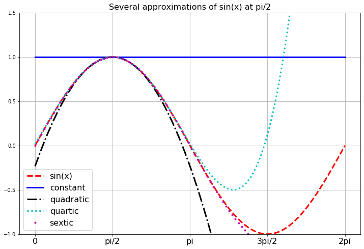

Figure 1.2: Taylor Series approximations of the sine function.

Exercise 1.35 Repeat the previous exercise for the functions \[\begin{eqnarray} f(x) &= \cos(x) \text{ centered at } x_0 = \pi \\ f(x) &= \ln(x) \text{ centered at } x_0 = 1 \end{eqnarray}\]

Exercise 1.36 Approximate $\cos(3)$ using a Taylor Series.

Exercise 1.37 Approximate $\ln(1.1)$ using a Taylor Series.

Example 1.4 Let’s conclude this brief section by examining an interesting example. Consider the function \[ f(x) = \frac{1}{1-x}. \] If we build a Taylor Series centered at $x_0 = 0$ (i.e. the Maclaurin Series) it isn’t too hard to show that we get \[ f(x) = 1 + x + x^2 + x^3 + x^4 + x^5 + \cdots \] (you should stop now and verify this!). However, if we plot the function $f(x)$ along with several successive approximations for $f(x)$ we find that beyond $x=1$ we don’t get the correct behavior of the function (see Figure 1.3). More specifically, we cannot get the Taylor Series to change behavior across the vertical asymptote of the function at $x=1$. This example is meant to point out the fact that a Taylor Series will only ever make sense near the point at which you center the expansion. For the function $f(x) = \frac{1}{1-x}$ centered at $x_0 = 0$ we can only get good approximations within the interval $x \in (-1,1)$ and no further.

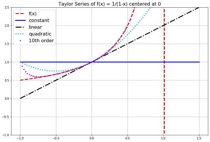
Figure 1.3: Several Taylor Series approximations of the function $f(x) = 1/(1-x)$.

In the previous example we saw that we cannot always get approximations from Taylor Series that are good everywhere. For every Taylor Series there is a domain of convergence where the Taylor Series actually makes sense and gives good approximations. While it is beyond the scope of this section to give all of the details for finding the domain of convergence for a Taylor Series, a good heuristic is to observe that a Taylor Series will only give reasonable approximations of a function from the center of the series to the nearest asymptote. The domain of convergence is typically symmetric about the center as well. For example:

If we were to build a Taylor Series approximation for the function $f(x) = \ln(x)$ centered at the point $x_0 = 1$ then the domain of convergence should be $x \in (0,2)$ since there is a vertical asymptote for the natural logarithm function at $x=0$.
If we were to build a Taylor Series approximation for the function $f(x) = \frac{5}{2x-3}$ centered at the point $x_0 = 4$ then the domain of convergence should be $x \in (1.5, 6.5)$ since there is a vertical asymptote at $x=1.5$ and the distance from $x_0 = 4$ to $x=1.5$ is 2.5 units.
If we were to build a Taylor Series approximation for the function $f(x) = \frac{1}{1+x^2}$ centered at the point $x_0 = 0$ then the domain of convergence should be $x \in (-1,1)$. This may seem quite odd (and perhaps quite surprising!) but let’s think about where the nearest asymptote might be. To find the asymptote we need to solve $1+x^2 = 0$ but this gives us the values $x = \pm i$. In the complex plane, the numbers $i$ and $-i$ are 1 unit away from $x_0 = 0$, so the “asymptote” isn’t visible in a real-valued plot but it is still only one unit away. Hence the domain of convergence is $x \in (-1,1)$. You should pause now and build some plots to show yourself that this indeed appears to be true.

A Taylor Series will give good approximations to the function within the domain of convergence, but will give garbage outside of it. For more details about the domain of convergence of a Taylor Series you can refer to the Taylor Series section of the online Active Calculus Textbook [2].

1.5 Approximation Error with Taylor Series

The great thing about Taylor Series is that they allow for the representation of potentially very complicated functions as polynomials – and polynomials are easily dealt with on a computer since they involve only addition, subtraction, multiplication, division, and integer powers. The down side is that the order of the polynomial is infinite. Hence, every time we use a Taylor series on a computer we are actually going to be using a Truncated Taylor Series where we only take a finite number of terms. The idea here is simple in principle:

If a function $f(x)$ has a Taylor Series representation it can be written as an infinite sum.
Computers can’t do infinite sums.
So stop the sum at some point $n$ and throw away the rest of the infinite sum.
Now $f(x)$ is approximated by some finite sum so long as you stay pretty close to $x = x_0$,
and everything that we just chopped off of the end is called the remainder for the finite sum.

Let’s be a bit more concrete about it. The Taylor Series for $f(x) = e^x$ centered at $x_0 = 0$ is \[ e^x = 1 + x + \frac{x^2}{2!} + \frac{x^3}{3!} + \frac{x^4}{4!} + \cdots. \]

$0^{th}$ Order Approximation of $f(x) = e^x$:: If we want to use a zeroth-order (constant) approximation of $f(x) = e^x$ then we only take the first term in the Taylor Series and the rest is not used for the approximation \[ e^x = \underbrace{1}_{\text{$0^{th}$ order approximation}} + \underbrace{x + \frac{x^2}{2!} + \frac{x^3}{3!} + \frac{x^4}{4!} + \cdots}_{\text{remainder}}. \] Therefore we would approximate $e^x$ as $e^x \approx 1$ for values of $x$ that are close to $x_0 = 0$. Furthermore, for small values of $x$ that are close to $x_0 = 0$ the largest term in the remainder is $x$ (since for small values of $x$ like 0.01, $x^2$ will be even smaller, $x^3$ even smaller than that, etc). This means that if we use a $0^{th}$ order approximation for $e^x$ then we expect our error to be about the same size as $x$. It is common to then rewrite the truncated Taylor Series as \[ \text{$0^{th}$ order approximation: } e^x \approx 1 + \mathcal{O}(x) \] where $\mathcal{O}(x)$ (read “Big-O of $x$”) tells us that the expected error for approximations close to $x_0 = 0$ is about the same size as $x$.
$1^{st}$ Order Approximation of $f(x) = e^x$:: If we want to use a first-order (linear) approximation of $f(x) = e^x$ then we gather the $0^{th}$ order and $1^{st}$ order terms together as our approximation and the rest is the remainder \[ e^x = \underbrace{1 + x}_{\text{$1^{st}$ order approximation}} + \underbrace{\frac{x^2}{2!} + \frac{x^3}{3!} + \frac{x^4}{4!} + \cdots}_{\text{remainder}}. \] Therefore we would approximate $e^x$ as $e^x \approx 1+x$ for values of $x$ that are close to $x_0 = 0$. Furthermore, for values of $x$ very close to $x_0 = 0$ the largest term in the remainder is the $x^2$ term. Using Big-O notation we can write the approximation as \[ \text{$1^{st}$ order approximation: } e^x \approx 1 + x + \mathcal{O}(x^2). \] Notice that we don’t explicitly say what the coefficient is for the $x^2$ term. Instead we are just saying that using the linear function $y=1+x$ to approximate $e^x$ for values of $x$ near $x_0=0$ will result in errors that are proportional to $x^2$.
$2^{nd}$ Order Approximation of $f(x) = e^x$:: If we want to use a second-order (quadratic) approximation of $f(x) = e^x$ then we gather the $0^{th}$ order, $1^{st}$ order, and $2^{nd}$ order terms together as our approximation and the rest is the remainder \[ e^x = \underbrace{1 + x + \frac{x^2}{2!}}_{\text{$2^{nd}$ order approximation}} + \underbrace{\frac{x^3}{3!} + \frac{x^4}{4!} + \cdots}_{\text{remainder}}. \] Therefore we would approximate $e^x$ as $e^x \approx 1+x+\frac{x^2}{2}$ for values of $x$ that are close to $x_0 = 0$. Furthermore, for values of $x$ very close to $x_0 = 0$ the largest term in the remainder is the $x^3$ term. Using Big-O notation we can write the approximation as \[ \text{$2^{nd}$ order approximation: } e^x \approx 1 + x + \frac{x^2}{2} + \mathcal{O}(x^3). \] Again notice that we don’t explicitly say what the coefficient is for the $x^3$ term. Instead we are just saying that using the quadratic function $y=1+x+\frac{x^2}{2}$ to approximate $e^x$ for values of $x$ near $x_0=0$ will result in errors that are proportional to $x^3$.

For the function $f(x) = e^x$ the idea of approximating the amount of approximation error by truncating the Taylor Series is relatively straight forward: if we want an $n^{th}$ order polynomial approximation of $e^x$ near $x_0 = 0$ then \[ e^x = 1 + x + \frac{x^2}{2!} + \frac{x^3}{3!} + \frac{x^4}{4!} + \cdots + \frac{x^n}{n!} + \mathcal{O}(x^{n+1}) \] meaning that we expect the error to be proportional to $x^{n+1}$.

Keep in mind that this sort of analysis is only good for values of $x$ that are very close to the center of the Taylor Series. If you are making approximations that are too far away then all bets are off.

Exercise 1.38 Let’s make the previous discussion a bit more concrete. We know the Taylor Series for $f(x) = e^x$ quite well at this point so let’s use it to approximate the value of $f(0.1) = e^{0.1}$ with different order polynomials. Notice that $x=0.1$ is pretty close to the center of the Taylor Series $x_0 = 0$ so this sort of approximation is reasonable.

Using np.exp(0.1) we have Python’s approximation $e^{0.1} \approx$ np.exp(0.1) $=1.1051709181$.

Fill in the blanks in the table.

Taylor Series	Approximation	Absolute Error	Expected Error
$0^{th}$ Order	$1$	$\|e^{0.1}-1\| = 0.1051709181$	$\mathcal{O}(x) = 0.1$
$1^{st}$ Order	$1.1$	$\|e^{0.1}-1.1\| = 0.0051709181$	$\mathcal{O}(x^2) = 0.1^2 = 0.01$
$2^{nd}$ Order	$1.105$
$3^{rd}$ Order
$4^{th}$ Order
$5^{th}$ Order

Observe in the previous exercise that the actual absolute error is always less than the expected error. Using the first term in the remainder to estimate the approximation error of truncating a Taylor Series is crude but very easy to implement.

Theorem 1.1 The approximation error when using a truncated Taylor Series is roughly proportional to the size of the next term in the Taylor Series.

Exercise 1.39 Next we will examine the approximation error for the sine function near $x_0 = 0$. We know that the sine function has the Taylor Series centered at $x_0 = 0$ as \[ \sin(x) = x - \frac{x^3}{3!} + \frac{x^5}{5!} - \frac{x^7}{7!} + \cdots. \]

A linear approximation of $\sin(x)$ near $x_0 = 0$ is $\sin(x) = x + \mathcal{O}(x^3)$.
1. Use the linear approximation formula to approximate $\sin(0.2)$.
2. What does “$\mathcal{O}(x^3)$” mean about the approximation of $\sin(0.2)$?
  (Take note that we ignore the minus sign on the approximation error since we are really only interested in absolute error (i.e. we don’t care if we overshoot or undershoot).)
Notice that there are no quadratic terms in the Taylor Series so there is no quadratic approximation for $\sin(x)$ near $x_0 =0$.
A cubic approximation of $\sin(x)$ near $x_0 = 0$ is $\sin(x) = ?? - ?? + \mathcal{O}(??)$.
1. Fill in the question marks in the cubic approximation formula.
2. Use the cubic approximation formula to approximate $\sin(0.2)$.
3. What is the approximation error for your approximation?
What is the next approximation formula for $\sin(x)$ near $x_0 = 0$? Use it to approximate $\sin(0.2)$, and give the expected approximation error.
Now let’s check all of our answers against what Python says we should get for $\sin(0.2)$. If you use np.sin(0.2) you should get $\sin(0.2) \approx$ np.sin(0.2) $=0.1986693308$. Fill in the blanks in the table below and then discuss the quality of our error approximations.

Taylor Series	Estimated Error	Actual Absolute Error
$1^{st}$ Order	$\mathcal{O}(x^3) = 0.2^3 = 0.008$	$0.001330669205$
$3^{rd}$ Order
$5^{th}$ Order
$7^{th}$ Order
$9^{th}$ Order

What observations do you make about the estimate of the approximation error and the actual approximation error?

Exercise 1.40 What if we want an approximation of $\ln(1.1)$ and we want that approximation to be within 5 decimal places. The number 1.1 is very close to 1 and we know that $\ln(1) = 0$. Hence, it seems like a good idea to build a Taylor Series approximation for $\ln(x)$ centered at $x_0 = 1$ to solve this problem.

Complete the table of derivatives below to get the Taylor coefficients for the Taylor Series of $\ln(x)$ centered at $x_0 = 1$.

Order of Derivative	Derivative	Value at $x_0 = 1$	Taylor Coefficient
0	$\ln(x)$	0	0
1	$\frac{1}{x} = x^{-1}$	1	1
2	$-x^{-2}$	$-1$	$\frac{-1}{2!} = -\frac{1}{2}$
3	$2x^{-3}$	2	$\frac{2}{3!} = \frac{1}{3}$
4	$-6x^{-4}$	$-6$
5
6
$\vdots$	$\vdots$	$\vdots$	$\vdots$

Based on what you did in part (a), complete the Taylor Series for $\ln(x)$ centered at $x_0 = 1$. \[ \ln(x) = 0 + 1(x-1) - \frac{1}{2}(x-1)^2 + \frac{1}{3}(x-1)^3 - \frac{??}{??}(x-1)^4 + \frac{??}{??}(x-1)^5 + \cdots. \]
The $n^{th}$ order Taylor approximation of $\ln(x)$ near $x_0 = 1$ is given below. What is the order of the estimated approximation error? \[ \ln(x) = (x-1) - \frac{(x-1)^2}{2} + \frac{(x-1)^3}{3} - \cdots + \frac{(-1)^{n-1} (x-1)^n}{n} + \mathcal{O}(???) \]
Finally we want to get an approximation for $\ln(1.1)$ accurate to 5 decimal places (or better). What is the minimum number of terms we expect to need from the Taylor Series? Support your answer mathematically.
Use Python’s np.log(1.1) to get an approximation for $\ln(1.1)$ and then numerically verify your answer to part (d).

Exercise 1.41 In the previous problem you found an approximation for $\ln(1.1)$ to 5 decimal places. In doing so you had to build a Taylor Series at a well-known point nearby 1.1 and then use our approximation of the error to determine the number of terms to keep in the approximation. In this exercise we want an approximation of $\cos\left( \frac{\pi}{2} + 0.05 \right)$. To do so you should build a Taylor Series for the cosine function centered at an appropriate point, determine an estimate for the approximation error, and then use that estimate to determine the number of terms to keep in the approximation.

1.6 Exercises

1.6.1 Coding Exercises

The first several exercises here are meant for you to practice and improve your coding skills. If you are stuck on any of the coding then I recommend that you have a look at Appendix A. Please refrain from Googling anything on these problems. The point is to struggle through the code, get it wrong many times, debug, and then to eventually have working code.

Exercise 1.42 (This problem is modified from [3])
If we list all of the numbers below 10 that are multiples of 3 or 5 we get 3, 5, 6, and 9. The sum of these multiples is 23. Write code to find the sum of all the multiples of 3 or 5 below 1000. Your code needs to run error free and output only the sum.

Exercise 1.43 (This problem is modified from [3])
Each new term in the Fibonacci sequence is generated by adding the previous two terms. By starting with 1 and 2, the first 10 terms will be: \[1, 1, 2, 3, 5, 8, 13, 21, 34, 55, \dots\] By considering the terms in the Fibonacci sequence whose values do not exceed four million, write code to find the sum of the even-valued terms. Your code needs to run error free and output only the sum.

Exercise 1.44 Write computer code that will draw random numbers from the unit interval $[0,1]$, distributed uniformly (using Python’s np.random.rand()), until the sum of the numbers that you draw is greater than 1. Keep track of how many numbers you draw. Then write a loop that does this process many many times. On average, how many numbers do you have to draw until your sum is larger than 1?

Hint #1:: Use the np.random.rand()command to draw a single number from a uniform distribution with bounds $(0,1)$.
Hint #2:: You should do this more than 1,000,000 times to get a good average …and the number that you get should be familiar!

Exercise 1.45 My favorite prime number is 8675309. Yep. Jenny’s phone number is prime! Write a script that verifies this fact.

Hint:: You only need to check divisors as large as the square root of 8675309 (why).

Exercise 1.46 (This problem is modified from [3])
Write a function called that accepts an integer and returns a binary variable:

0 = not prime,
1 = prime.

Next write a script to find the sum of all of the prime numbers less than 1000.

Hint:: Remember that a prime number has exactly two divisors: 1 and itself. You only need to check divisors as large as the square root of $n$. Your script should probably be smart enough to avoid all of the non-prime even numbers.

Exercise 1.47 (This problem is modified from [3])
The sum of the squares of the first ten natural numbers is, \[1^2 + 2^2 + \dots + 10^2 = 385\] The square of the sum of the first ten natural numbers is, \[(1 + 2 + \dots + 10)^2 = 55^2 = 3025\] Hence the difference between the square of the sum of the first ten natural numbers and the sum of the squares is $3025 - 385 = 2640$.

Write code to find the difference between the square of the sum of the first one hundred natural numbers and the sum of the squares. Your code needs to run error free and output only the difference.

Exercise 1.48 (This problem is modified from [3])
The prime factors of $13195$ are $5, 7, 13$ and $29$. Write code to find the largest prime factor of the number $600851475143$? Your code needs to run error free and output only the largest prime factor.

Exercise 1.49 (This problem is modified from [3])
The number 2520 is the smallest number that can be divided by each of the numbers from 1 to 10 without any remainder. Write code to find the smallest positive number that is evenly divisible by all of the numbers from 1 to 20?

Hint: You will likely want to use modular division for this problem.

Exercise 1.50 The following iterative sequence is defined for the set of positive integers: \[\begin{aligned} & n \to \frac{n}{2} \quad \text{(n is even)} \\ & n \to 3n + 1 \quad \text{(n is odd)} \end{aligned}\] Using the rule above and starting with $13$, we generate the following sequence: \[13 \to 40 \to 20 \to 10 \to 5 \to 16 \to 8 \to 4 \to 2 \to 1\] It can be seen that this sequence (starting at 13 and finishing at 1) contains 10 terms. Although it has not been proved yet (Collatz Problem), it is thought that all starting numbers finish at 1. This has been verified on computers for massively large starting numbers, but this does not constitute a proof that it will work this way for all starting numbers.

Write code to determine which starting number, under one million, produces the longest chain. NOTE: Once the chain starts the terms are allowed to go above one million.

1.6.2 Applying What You’ve Learned

Exercise 1.51 (This problem is modified from [4])
Sometimes floating point arithmetic does not work like we would expect (and hope) as compared to by-hand mathematics. In each of the following problems we have a mathematical problem that the computer gets wrong. Explain why the computer is getting these wrong.

Mathematically we know that $\sqrt{5}^2$ should just give us 5 back. In Python type np.sqrt(5)**2 == 5. What do you get and why do you get it?
Mathematically we know that $\left( \frac{1}{49} \right) \cdot 49$ should just be 1. In Python type (1/49)*49 == 1. What do you get and why do you get it?
Mathematically we know that $e^{\ln(3)}$ should just give us 3 back. In Python type np.exp(np.log(3)) == 3. What do you get and why do you get it?
Create your own example of where Python gets something incorrect because of floating point arithmetic.

Exercise 1.52 (This problem is modified from [4])
In the 1999 movie Office Space, a character creates a program that takes fractions of cents that are truncated in a bank’s transactions and deposits them to his own account. This is idea has been attempted in the past and now banks look for this sort of thing. In this problem you will build a simulation of the program to see how long it takes to become a millionaire.

Assumptions:

Assume that you have access to 50,000 bank accounts.
Assume that the account balances are uniformly distributed between $100 and $100,000.
Assume that the annual interest rate on the accounts is 5% and the interest is compounded daily and added to the accounts, except that fractions of cents are truncated.
Assume that your illegal account initially has a $0 balance.

Your Tasks:

Explain what the code below does.

import numpy as np
accounts = 100 + (100000-100) * np.random.rand(50000,1);
accounts = np.floor(100*accounts)/100;

By hand (no computer) write the mathematical steps necessary to increase the accounts by (5/365)% per day, truncate the accounts to the nearest penny, and add the truncated amount into an account titled “illegal.”
Write code to complete your plan from part (b).
Using a while loop, iterate over your code until the illegal account has accumulated $1,000,000. How long does it take?

Exercise 1.53 (This problem is modified from [4])
In the 1991 Gulf War, the Patriot missle defense system failed due to roundoff error. The troubles stemmed from a computer that performed the tracking calculations with an internal clock whose integer values in tenths of a second were converted to seconds by multiplying by a 24-bit binary approximation to $\frac{1}{10}$: \[0.1_{10} \approx 0.00011001100110011001100_2.\]

Convert the binary number above to a fraction by hand (common denominators would be helpful).
The approximation of $\frac{1}{10}$ given above is clearly not equal to $\frac{1}{10}$. What is the absolute error in this value?
What is the time error, in seconds, after 100 hours of operation?
During the 1991 war, a Scud missile traveled at approximately Mach 5 (3750 mph). Find the distance that the Scud missle would travel during the time error computed in (c).

Exercise 1.54 Find the Taylor Series for $f(x) = \frac{1}{\ln(x)}$ centered at the point $x_0 = e$. Then use the Taylor Series to approximate the number $\frac{1}{\ln(3)}$ to 4 decimal places.

Exercise 1.55 In this problem we will use Taylor Series to build approximations for the irrational number $\pi$.

Write the Taylor series centered at $x_0=0$ for the function \[ f(x) = \frac{1}{1+x}. \]
Now we want to get the Taylor Series for the function $g(x) = \frac{1}{1+x^2}$. It would be quite time consuming to take all of the necessary derivatives to get this Taylor Series. Instead we will use our answer from part (a) of this problem to shortcut the whole process.
1. Substitute $x^2$ for every $x$ in the Taylor Series for $f(x) = \frac{1}{1+x}$.
2. Make a few plots to verify that we indeed now have a Taylor Series for the function $g(x) = \frac{1}{1+x^2}$.
Recall from Calculus that \[ \int \frac{1}{1+x^2} dx = \arctan(x). \] Hence, if we integrate each term of the Taylor Series that results from part (b) we should have a Taylor Series for $\arctan(x)$.¹
Now recall the following from Calculus:

$\tan(\pi/4) = 1$
so $\arctan(1) = \pi/4$
and therefore $\pi = 4\arctan(1)$.

Let’s use these facts along with the Taylor Series for $\arctan(x)$ to approximate $\pi$: we can just plug in $x=1$ to the series, add up a bunch of terms, and then multiply by 4. Write a loop in Python that builds successively better and better approximations of $\pi$. Stop the loop when you have an approximation that is correct to 6 decimal places.

Exercise 1.56 In this problem we will prove the famous (and the author’s favorite) formula \[e^{i\theta} = \cos(\theta) + i \sin(\theta).\] This is known as Euler’s formula after the famous mathematician Leonard Euler. Show all of your work for the following tasks.

Write the Taylor series for the functions $e^x$, $\sin(x)$, and $\cos(x)$.
Replace $x$ with $i\theta$ in the Taylor expansion of $e^x$. Recall that $i = \sqrt{-1}$ so $i^2 = -1$, $i^3 = -i$, and $i^4 = 1$. Simplify all of the powers of $i\theta$ that arise in the Taylor expansion. I’ll get you started: \[\begin{aligned} e^x &= 1 + x + \frac{x^2}{2} + \frac{x^3}{3!} + \frac{x^4}{4!} + \frac{x^5}{5!} + \cdots \\ e^{i\theta} &= 1 + (i\theta) + \frac{(i\theta)^2}{2!} + \frac{(i\theta)^3}{3!} + \frac{(i\theta)^4}{4!} + \frac{(i\theta)^5}{5!} + \cdots \\ &= 1 + i\theta + i^2 \frac{\theta^2}{2!} + i^3 \frac{\theta^3}{3!} + i^4 \frac{\theta^4}{4!} + i^5 \frac{\theta^5}{5!} + \cdots \\ &= \ldots \text{ keep simplifying ... } \ldots \end{aligned}\]
Gather all of the real terms and all of the imaginary terms together. Factor the $i$ out of the imaginary terms. What do you notice?
Use your result from part (c) to prove that $e^{i\pi} + 1 = 0$.

Exercise 1.57 In physics, the relativistic energy of an object is defined as \[ E_{rel} = \gamma mc^2 \] where \[ \gamma = \frac{1}{\sqrt{1 - \frac{v^2}{c^2}}}. \] In these equations, $m$ is the mass of the object, $c$ is the speed of light ($c \approx 3 \times 10^8$m/s), and $v$ is the velocity of the object. For an object of fixed mass (m) we can expand the Taylor Series centered at $v=0$ for $E_{rel}$ to get \[ E_{rel} = mc^2 + \frac{1}{2} mv^2 + \frac{3}{8} \frac{mv^4}{c^2} + \frac{5}{16} \frac{mv^6}{c^4} + \cdots. \]

What do we recover if we consider an object with zero velocity?
Why might it be completely reasonable to only use the quadratic approximation \[ E_{rel} = mc^2 + \frac{1}{2} mv^2 \] for the relativistic energy equation?²
(some physics knowledge required) What do you notice about the second term in the Taylor Series approximation of the relativistic energy function?
Show all of the work to derive the Taylor Series centered at $v = 0$ given above.

Exercise 1.58 (The Python Caret Operator)Now that you’re used to using Python to do some basic computations you are probably comfortable with the fact that the caret, ^, does NOT do exponentiation like it does in many other programming languages. But what does the caret operator do? That’s what we explore here.

Consider the numbers $9$ and $5$. Write these numbers in binary representation. We are going to use four bits to represent each number (it is ok if the first bit happens to be zero). \[\begin{aligned} 9 &=& \underline{\hspace{0.2in}} \, \underline{\hspace{0.2in}} \, \underline{\hspace{0.2in}} \, \underline{\hspace{0.2in}} \\ 5 &=& \underline{\hspace{0.2in}} \, \underline{\hspace{0.2in}} \, \underline{\hspace{0.2in}} \, \underline{\hspace{0.2in}} \end{aligned}\]
Now go to Python and evaluate the expression 9^5. Convert Python’s answer to a binary representation (again using four bits).
Make a conjecture: How do we go from the binary representations of $a$ and $b$ to the binary representation for Python’s a^b for numbers $a$ and $b$? Test and verify your conjecture on several different examples and then write a few sentences explaining what the caret operator does in Python.

References

[2]

M. Boelkins, “Active calculus.” https://activecalculus.org/single/frontmatter.html, 2018.

[3]

“ProjectEuler.net.” https://projecteuler.net/.

[4]

A. Greenbaum and T. Chartier, Numerical methods: Design, analysis, and computer implementation of algorithms. Princeton University Press, 2012.

There are many reasons why integrating an infinite series term by term should give you a moment of pause. For the sake of this problem we are doing this operation a little blindly, but in reality we should have verified that the infinite series actually converges uniformly. ↩︎
This is something that people in physics and engineering do all the time – there is some complicated nonlinear relationship that they wish to use, but the first few terms of the Taylor Series captures almost all of the behavior since the higher-order terms are very very small.↩︎

Taylor Series	Approximation	Absolute Error	Expected Error
\(0^{th}\) Order	\(1\)	\(\|e^{0.1}-1\| = 0.1051709181\)	\(\mathcal{O}(x) = 0.1\)
\(1^{st}\) Order	\(1.1\)	\(\|e^{0.1}-1.1\| = 0.0051709181\)	\(\mathcal{O}(x^2) = 0.1^2 = 0.01\)
\(2^{nd}\) Order	\(1.105\)
\(3^{rd}\) Order
\(4^{th}\) Order
\(5^{th}\) Order

Taylor Series	Estimated Error	Actual Absolute Error
\(1^{st}\) Order	\(\mathcal{O}(x^3) = 0.2^3 = 0.008\)	\(0.001330669205\)
\(3^{rd}\) Order
\(5^{th}\) Order
\(7^{th}\) Order
\(9^{th}\) Order

Order of Derivative	Derivative	Value at \(x_0 = 1\)	Taylor Coefficient
0	\(\ln(x)\)	0	0
1	\(\frac{1}{x} = x^{-1}\)	1	1
2	\(-x^{-2}\)	\(-1\)	\(\frac{-1}{2!} = -\frac{1}{2}\)
3	\(2x^{-3}\)	2	\(\frac{2}{3!} = \frac{1}{3}\)
4	\(-6x^{-4}\)	\(-6\)
5
6
\(\vdots\)	\(\vdots\)	\(\vdots\)	\(\vdots\)

Approximation Function	Value at \(x=1\)	Absolute Error
Constant	1	\(\| 2.71828... - 1\| \approx 1.71828...\)
Linear	1+1=2	\(\|2.71828... - 2\| \approx 0.71828...\)
Quadratic
Cubic
Quartic
Quintic